本文介绍了上帝之心的算法及其Python实现,使用Python语言的性能分析工具测算性能瓶颈,将算法最耗时的部分重构至CUDA C语言在纯GPU上运行,利用GPU核心更多并行更快的优势显著提高算法运算速度,实现了结果不变的情况下将耗时缩短五十倍的目标。
2.1 简单Python画曼德勃罗特集算法
2.1.1 “上帝之心”的由来
曼德勃罗特集是一个几何图形,曾被称为“上帝的指纹”。

只要计算的点足够多,不管把图案放大多少倍,都能显示出更加复杂的局部,这些局部既与整体不同,又有某种相似的地方。
图案具有无穷无尽的细节和自相似性。如图所示形产生过程,其中后一个图均是前一个图的某一局部放大:
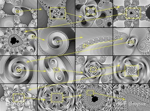
来源:百度百科
2.2.2 简单py算法实现
跟任意GPT要一个简单Python实现的曼德勃罗特集算法,可以得到以下源码:
def simple_mandelbrot(width, height, real_low, real_high, imag_low, imag_high, max_iters, upper_bound):real_vals = np.linspace(real_low, real_high, width)imag_vals = np.linspace(imag_low, imag_high, height) mandelbrot_graph = np.ones((height, width), dtype=np.float32) for x in range(width):for y in range(height):c = np.complex64(real_vals[x] + imag_vals[y] * 1j)z = np.complex64(0) for i in range(max_iters):z = z ** 2 + c if np.abs(z) > upper_bound:mandelbrot_graph[y, x] = 0break return mandelbrot_graph加上具体的图片大小,实部虚部,迭代次数,发散阈值,进行计算,并记录计算时间,且保存图像,记录保存时间。
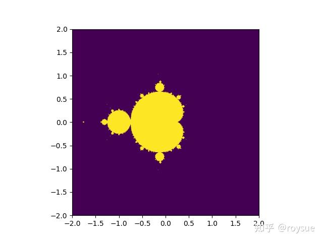
if __name__ == '__main__':t1 = time()mandel = simple_mandelbrot(512, 512, -2, 2, -2, 2, 256, 2.5)t2 = time()mandel_time = t2 - t1t1 = time()fig = plt.figure(1)plt.imshow(mandel, extent=(-2, 2, -2, 2))plt.savefig('mandelbrot.png', dpi=fig.dpi)t2 = time()dump_time = t2 - t1print('It took {} seconds to calculate the Mandelbrot graph.'.format(mandel_time))print('It took {} seconds to dump the image.'.format(dump_time))在笔者的i5-13490F的CPU上,Python3.12.3版本,输出结果是:
~/Desktop/EXAMPLES/02$ ../bin/python mandelbrot.py
It took 3.529670000076294 seconds to calculate the Mandelbrot graph.
It took 0.06651782989501953 seconds to dump the image.
计算过程耗时3.53秒,存成图片耗时0.067秒。图片如图:
2.2 cProfile性能分析算法函数瓶颈
2.2.1 函数粒度分析性能瓶颈
Python 的 cProfile 模块是一个内置的性能分析工具(Profiler),用于统计代码中各个函数的执行时间、调用次数等详细信息,帮助开发者找出程序的性能瓶颈。
主要功能特点包括:
- 统计每个函数的调用次数和时间:记录函数的总执行时间(包括子函数调用)和单独执行时间(不包括子函数)。
- 生成性能报告:以表格形式输出结果,方便分析热点代码。
- 低开销:相比 profile 模块(纯 Python 实现),cProfile 是 C 语言实现的,对程序运行速度影响较小。
使用-m参数调用cProfile模块,按照累计运行时间降序排列-s cumtime,结果重定向至mandelbrot_cProfile.txt文件。
$ ../bin/python -m cProfile -s cumtime mandelbrot.py > mandelbrot_cProfile.txt最终结果输出前20行可以得知,mandelbrot.py:10(simple_mandelbrot)就调用了1次,耗时4.016秒,为tottime指标最高的单一函数。
$ head -20  mandelbrot_cProfile.txt
It took 4.01598596572876 seconds to calculate the Mandelbrot graph.
It took 0.10479903221130371 seconds to dump the image.1272295 function calls (1250243 primitive calls) in 4.610 secondsOrdered by: cumulative timencalls  tottime  percall  cumtime  percall filename:lineno(function)65/2    0.000    0.000    4.503    2.252 text.py:926(get_window_extent)101/2    0.002    0.000    4.503    2.252 text.py:358(_get_layout)1    4.016    4.016    4.016    4.016 mandelbrot.py:10(simple_mandelbrot)32    0.001    0.000    0.632    0.020 __init__.py:1(<module>)349/7    0.001    0.000    0.424    0.061 <frozen importlib._bootstrap>:1349(_find_and_load)346/7    0.001    0.000    0.424    0.061 <frozen importlib._bootstrap>:1304(_find_and_load_unlocked)331/7    0.001    0.000    0.423    0.060 <frozen importlib._bootstrap>:911(_load_unlocked)
PS: tottime(直接运行时间)表示函数本身运行的时间,不包括调用其他函数的时间,它是函数内部执行代码的时间总和,不考虑子函数的执行时间。而 cumtime(累积运行时间)表示函数及其所有子函数运行的总时间,它包括函数本身的时间(tottime)加上所有被该函数调用的子函数的时间总和。
2.2.2 逐行耗时分析性能瓶颈
cProfile模块最小粒度为函数,如果想逐行分析,可以使用line_profiler模块。
line_profiler 是一个第三方库,可以显示每行代码的执行时间、次数和耗时占比。
首先安装该模块:
$ ../bin/pip install line_profiler
Collecting line_profilerDownloading line_profiler-4.2.0-cp312-cp312-manylinux_2_17_x86_64.manylinux2014_x86_64.whl.metadata (34 kB)
Downloading line_profiler-4.2.0-cp312-cp312-manylinux_2_17_x86_64.manylinux2014_x86_64.whl (720 kB)━━━━━━━━━━━━━━━━━━━━━━━━━━━━━━━━━━━━━━━━ 720.1/720.1 kB 3.9 MB/s eta 0:00:00
Installing collected packages: line_profiler
Successfully installed line_profiler-4.2.0然后在需要分析的函数名称前加上@profile装饰器。
@profile
def simple_mandelbrot(width, height, real_low, real_high, imag_low, imag_high, max_iters, upper_bound):real_vals = np.linspace(real_low, real_high, width)imag_vals = np.linspace(imag_low, imag_high, height)...最后使用kernprof命令行工具运行脚本,-l 表示逐行分析,-v 表示运行后立即显示结果。
~/Desktop/EXAMPLES/02$ ../bin/kernprof -l -v mandelbrot.py
It took 8.354495286941528 seconds to calculate the Mandelbrot graph.
It took 0.07214522361755371 seconds to dump the image.
Wrote profile results to mandelbrot.py.lprof
Timer unit: 1e-06 sTotal time: 6.02906 s
File: mandelbrot.py
Function: simple_mandelbrot at line 9Line #      Hits         Time  Per Hit   % Time  Line Contents
==============================================================9 @profile 10 def simple_mandelbrot(width, height, real_low, real_high, imag_low, imag_high, max_iters, upper_bound):11 1 57.4 57.4 0.0 real_vals = np.linspace(real_low, real_high, width)12 1 16.5 16.5 0.0 imag_vals = np.linspace(imag_low, imag_high, height)13 14 # we will represent members as 1, non-members as 0.15 1 274.7 274.7 0.0 mandelbrot_graph = np.ones((height, width), dtype=np.float32)16 17 513 53.5 0.1 0.0 for x in range(width):18 262656 28811.2 0.1 0.5 for y in range(height):19 262144 306395.3 1.2 5.1 c = np.complex64(real_vals[x] + imag_vals[y] * 1j)20 262144 75984.6 0.3 1.3 z = np.complex64(0)21 22 7282380 791951.4 0.1 13.1 for i in range(max_iters):23 7257560 1193944.6 0.2 19.8 z = z ** 2 + c24 25 7257560 3568029.4 0.5 59.2 if np.abs(z) > upper_bound:26 237324 40273.0 0.2 0.7 mandelbrot_graph[y, x] = 027 237324 23266.9 0.1 0.4 break28 29 1 1.0 1.0 0.0 return mandelbrot_graph使用line_profiler模块会拖慢函数,从3秒慢到了8秒。运行结果是函数逐行的耗时,其中: - Hits:该行执行次数 - Time:该行总耗时(微秒) - % Time:该行占函数总耗时的百分比。
耗时最多的三行,功能分别是控制每个像素点的迭代次数(max_iters 次)、曼德勃罗集的迭代公式(复数运算)、和检查曼德勃罗集(Mandelbrot)的逃逸条件(判断复数 z 的模是否超过阈值 upper_bound),耗时多的原因是执行次数过多,各执行了7,257,560 次,每次都要运行复数平方运算(z ** 2)和复数的模(np.abs(z))需要浮点计算。
for i in range(max_iters):z = z ** 2 + cif np.abs(z) > upper_bound:这三行代码的运算时间之和占整体的92.1%,如果优化这里可以显著降低算法运行时间,提高效率。
2.3 PyCUDA之gpuarray显卡跑算法
2.3.1 “Hello World”
跟任意GPT要个gpuarray的“Hello World”代码,可以得到类似如下代码。注释部分也是GPT添加的。
import numpy as np
#自动内存管理:使用 pycuda.autoinit 自动管理CUDA上下文,简化了代码,适合简单的脚本。
import pycuda.autoinit
#PyCUDA 提供了类似 NumPy 的接口,使得在 GPU 上进行数组操作非常直观和方便。
from pycuda import gpuarray
#创建主机数组:使用 NumPy 创建一个数组 host_data,包含元素 [1, 2, 3, 4, 5],数据类型为 float32。dtype=np.float32 确保数组的数据类型为单精度浮点数,这对于GPU计算很重要,因为 GPU 在处理浮点数时通常更高效。确保主机数组和GPU数组的数据类型一致(如 float32)可以避免潜在的错误和性能问题。
host_data = np.array([1,2,3,4,5] , dtype=np.float32)
#将主机数组传输到 GPU:使用 gpuarray.to_gpu() 方法将主机数组 host_data 传输到 GPU 上,并存储在 device_data 中。device_data 现在是一个GPU数组,存储在 GPU 的显存中。
device_data=gpuarray.to_gpu(host_data)
#在 GPU 上进行逐元素乘法操作:使用 2 * device_data 对 GPU 数组 device_data 中的每个元素乘以 2。这个操作在 GPU 上并行执行,速度比在 CPU 上逐元素操作快得多。结果存储在新的 GPU 数组 device_data_x2 中。
device_data_x2 = 2 * device_data
#将结果从 GPU 传输回主机,使用 .get() 方法将 GPU 数组 device_data_x2 中的数据传输回主机内存,并存储在 host_data_x2 中。host_data_x2 是一个 NumPy 数组,包含操作后的结果。
host_data_x2=device_data_x2.get()
print(host_data_x2)
运行一下,得到如下结果:
$ ../bin/python gpuarray.py
[ 2.  4.  6.  8. 10.]
这是我们第一段在显卡上直接运行代码。
需要注意的是,向显卡发送数据时,需要通过NumPy显示声明数据类型。这样做的好处有两个:
- 避免类型转换带来不必要的开销,消耗更多的计算时间或内存;
- 后续会用CUDA C语言来内联编写代码,必须为变量声明规定具体的类型,否则C代码无法工作,毕竟C是编译型语言
2.3.2 GPU和CPU工作原理的差异
前文的案例中,逐元素乘以常量的操作,是可以并行化运行的,因为一个元素的计算并不依赖其他任何元素的计算结果。
所以在gpuarray的线程上执行该操作时,PyCUDA可以将乘法操作转移至一个个单独的线程上,而不用像CPU一样一个接一个地串行计算。这也是GPU高吞吐的原因,CPU则是高性能。
- 可以将GPU类比于迅雷,每秒下载几兆的数据,倘若有延迟一两秒大家也不关心,大家更关心传输量大,此处“网很快、下载得快”的意思就是吞吐大,每秒多少兆。
- CPU类似于打网络游戏,延迟一般要求低于30ms,倘若延迟大于200ms网络游戏就几乎没有体验可言了,技能释放慢个几百毫秒结果就完全不同,但是丝毫不关心吞吐量,此处“网络很快”的意思就是延迟极低。
日常使用电脑的过程中,主要追求的也是低延迟。鼠标拖动的时候,肉眼不可以看到停顿,键盘按下去屏幕上立刻出现字符,桌面快捷方式双击后,程序窗口要立即出现,在程序之间切换要流畅自如毫无拖沓。
而什么场景需要显卡呢?典型场景,也是显卡迄今为止最为主要的工作内容,就是游戏画面渲染,一草一木、光影追踪,游戏两个最为核心的指标,画质和帧率,也就是渲染的画面的质量(像素点的多少)和每秒可以渲染多少张,此时评价显卡很快的意思就是,每秒出的图又细又多,也就是高吞吐。每秒出10张480p的图,相比每秒出100张1080p的图,玩的游戏体验不在一个次元上。
再来看一段GPU和CPU跑相同算法的速度对比。编写一段代码(time_calc.py),分别在CPU和GPU上运行同样的常量乘法计算,对比执行速度。
import numpy as np
import pycuda.autoinit
from pycuda import gpuarray
from time import time
#创建五千万个随机单精度浮点数
host_data = np.float32(np.random.random(50000000))
#CPU计算耗时
t1 = time()
host_data_2x = host_data * np.float32(2)
t2 = time()
print('total time to compute on CPU: %f' % (t2 - t1))
#传输到显卡进行计算耗时
device_data = gpuarray.to_gpu(host_data)
t1 = time()
device_data_2x = device_data * np.float32(2)
t2 = time()
#数据从显卡传回主机
from_device = device_data_2x.get()
#比较 CPU 和 GPU 的计算结果是否相同
print('total time to compute on GPU: %f' % (t2 - t1))
print('Is the host computation the same as the GPU computation? : {}'.format(np.allclose(from_device, host_data_2x)))
在笔者机器i5-13490F、RTX5060ti 12G上运行三次,对比差异:
$ ../bin/python time_calc.py
total time to compute on CPU: 0.043279
total time to compute on GPU: 0.058837
Is the host computation the same as the GPU computation? : True
$ ../bin/python time_calc.py
total time to compute on CPU: 0.047776
total time to compute on GPU: 0.058785
Is the host computation the same as the GPU computation? : True
$ ../bin/python time_calc.py
total time to compute on CPU: 0.046850
total time to compute on GPU: 0.057116
Is the host computation the same as the GPU computation? : True
可以发现CPU的速度几乎和GPU一样的快,这是什么原因呢?因为NumPy可以利用现代CPU中的SSE指令来加速计算,在某些场景中性能可以与GPU相媲美。
可以把浮点数的个数设置成五亿个:
host_data = np.float32(np.random.random(500000000))再运行三次对比差异:
$ ../bin/python time_calc.py
total time to compute on CPU: 0.437335
total time to compute on GPU: 0.263772
Is the host computation the same as the GPU computation? : True
$ ../bin/python time_calc.py
total time to compute on CPU: 0.436809
total time to compute on GPU: 0.056556
Is the host computation the same as the GPU computation? : True
$ ../bin/python time_calc.py
total time to compute on CPU: 0.438307
total time to compute on GPU: 0.060931
Is the host computation the same as the GPU computation? : True
可以看到在第二次、第三次运行时,GPU的耗时约为CPU的十分之一,并行提速效果显著。可以推理得到倘若数据量更大会提速更多。
那为什么第一次GPU耗时偏多呢?因为PyCUDA编写的代码中的CUDA逻辑部分第一次运行时需要使用NVCC编译器编译成字节码,以供PyCUDA调用,所以第一次运行时间会长一些;后续再次调用时,如果代码没有修改,则直接使用已经编译好的缓存即可,这与我们玩一些3A大作的游戏,第一次运行需要进行“着色器编译”是相同的原理。
2.4 PyCUDA之内联CUDA C算法提速
对gpuarray对象进行操作,默认会在纯GPU上执行,上一节对元素乘以2时,这个对象2会传输到GPU上,由GPU在显存中创建对象,在显卡的核心上并行计算。
如果操作涉及gpuarray与主机数据(或变量如numpy数组)的混合运算,PyCUDA会报错,因为它无法隐式决定数据位置。比如:
# 会报错!不能直接混合gpuarray和CPU创建的numpy数组
device_data_2x = device_data * np.ones(100)必须显式将数据放置在纯GPU(或纯CPU)上。那具体代码如何写呢?这里就可以引入ElementwiseKernel函数,直接内联CUDA C代码编程,追求最为设备原生的高性能。下面上案例(simple_element_kernel_example0.py):
import numpy as np
import pycuda.autoinit
from pycuda import gpuarray
from time import time
#用于创建元素级操作的CUDA内核
from pycuda.elementwise import ElementwiseKernel
host_data = np.float32(np.random.random(500000000))
# 定义一个CUDA元素级内核:输入参数:两个float指针(in和out),操作:将输入数组的每个元素乘以2,结果存入输出数组,内核名称:"gpu_2x_ker"
gpu_2x_ker = ElementwiseKernel("float *in, float *out","out[i] = 2*in[i];","gpu_2x_ker"
)
def speedcomparison():t1 = time()host_data_2x = host_data * np.float32(2)t2 = time()print('total time to compute on CPU: %f' % (t2 - t1))device_data = gpuarray.to_gpu(host_data)# 在GPU上分配与输入数组大小相同的空输出数组device_data_2x = gpuarray.empty_like(device_data)t1 = time()# 调用之前定义的CUDA内核在GPU上执行计算gpu_2x_ker(device_data, device_data_2x)t2 = time()from_device = device_data_2x.get()print('total time to compute on GPU: %f' % (t2 - t1))print('Is the host computation the same as the GPU computation? : {}'.format(np.allclose(from_device, host_data_2x)))
if __name__ == '__main__':speedcomparison()
这样包括输入的所有参数、运算符和输出,都是在纯GPU的设备里操作,达到设备级别的原生高性能。同样多运行几次,观察速度差异:
$ ../bin/python simple_element_kernel_example0.py
total time to compute on CPU: 0.431743
total time to compute on GPU: 0.565969
Is the host computation the same as the GPU computation? : True
$ ../bin/python simple_element_kernel_example0.py
total time to compute on CPU: 0.436628
total time to compute on GPU: 0.062304
Is the host computation the same as the GPU computation? : True
$ ../bin/python simple_element_kernel_example0.py
total time to compute on CPU: 0.433212
total time to compute on GPU: 0.055214
Is the host computation the same as the GPU computation? : True
同样可以观察到与前文一样的现象,首次运行CUDA C部分需要先用NVCC编译,再次运行速度才会获得显著提升。
PS:思考:前文的混合运算这样写:device_data_2x = device_data * device_data,可以吗?答案是可以的,这表示两个GPU数组(gpuarray)之间的逐元素乘法,PyCUDA会将乘法运算符转成CUDA C的乘法,这个操作会完全在纯GPU上并行执行。
2.5 纯GPU重构算法比CPU快五十倍
那最后的任务就是把耗时占92.1%的以下三行代码用CUDA C重写,使之充分利用显卡并行计算大吞吐的特性,进行充分的加速。
for i in range(max_iters):z = z ** 2 + cif np.abs(z) > upper_bound:算法开发和移植是当前工资最高的工作,可惜我不会,我只能问GPT。可悲的是,如果不会算法,连怎么调试,生成的结果对不对,模型有没有出现幻觉,都无法判断,毕竟在算法这个领域,GPT的能力大于自己。
幸亏我们的案例来自书籍,有作者调好的版本,同功能的CUDA C算法实现如下,可以说与Python的写法几乎一模一样:
mandelbrot_graph[i] = 1;
pycuda::complex<float> c = lattice[i];
pycuda::complex<float> z(0,0);
for (int j = 0; j < max_iters; j++)
{z = z*z + c; if(abs(z) > upper_bound){mandelbrot_graph[i] = 0;break;}
}
同样算法的各种参数也需要改变:
def gpu_mandelbrot(width, height, real_low, real_high, imag_low, imag_high, max_iters, upper_bound):# we set up our complex lattice as suchreal_vals = np.matrix(np.linspace(real_low, real_high, width), dtype=np.complex64)imag_vals = np.matrix(np.linspace(imag_high, imag_low, height), dtype=np.complex64) * 1jmandelbrot_lattice = np.array(real_vals + imag_vals.transpose(), dtype=np.complex64) # copy complex lattice to the GPU#gpuarray.to_gpu函数只能处理NumPy的array类型,所以发送到GPU之前要进行包装;mandelbrot_lattice_gpu = gpuarray.to_gpu(mandelbrot_lattice)# allocate an empty array on the GPU#gpuarray.empty函数在GPU上分配内存,指定大小、形状及类型,可以看作是C语言中的malloc函数;比C的优点是不需要惦记内存释放或回收,因为gpuarray对象在析构时会自动清理。mandelbrot_graph_gpu = gpuarray.empty(shape=mandelbrot_lattice.shape, dtype=np.float32)#注意CUDA C里的模板类型pycuda::complex和Python代码里的NumPy的Complex64是对应的,否则参数传递过去是无法解析的。比如CUDA C的int类型对应NumPy的int32类型,CUDA C的float类型对应NumPy的float32类型。另外,数组传递给CUDA C时,会被视为C指针。mandel_ker(mandelbrot_lattice_gpu, mandelbrot_graph_gpu, np.int32(max_iters), np.float32(upper_bound)) mandelbrot_graph = mandelbrot_graph_gpu.get() return mandelbrot_graph与原来的纯Python相比逻辑是一样的,只是多了各种数据格式的转换和映射,最后就是激动人心的测速环节,还是i5-13490F、RTX5060ti 12G的机器:
~/Desktop/EXAMPLES/02$ ../bin/python gpu_mandelbrot.py
It took 0.1877138614654541 seconds to calculate the Mandelbrot graph.
It took 0.09330153465270996 seconds to dump the image.
~/Desktop/EXAMPLES/02$ ../bin/python gpu_mandelbrot.py
It took 0.05863165855407715 seconds to calculate the Mandelbrot graph.
It took 0.07119488716125488 seconds to dump the image.
~/Desktop/EXAMPLES/02$ ../bin/python gpu_mandelbrot.py
It took 0.062407732009887695 seconds to calculate the Mandelbrot graph.
It took 0.06969809532165527 seconds to dump the image.
同理第一次运行,是NVCC编译花了一些时间,后面稳定在0.06秒左右的水平,从3.53秒到0.06秒,大概是59倍的性能提升。
当然,需要对比确认下生成的PNG图片是一致的。本章节的任务成功完成。通过这个实验相信大家对GPU特性的理解可以说是非常深刻了。
PS:最后又让deepseek帮助优化了一下代码,执行ds优化后的版本,生成同样的图,速度降到了0.0036秒,是书中代码的1/20,可见,优化是深不见底的学问。

- 代码等附件下载地址:https://github.com/r0ysue/5060STUDY
引用来源: - 《GPU编程实战(基于Python和CUDA)》、deepseek