训练和测试的规范写法
一、黑白图片的规范写法,以MNIST数据集为例
import torch
import torch.nn as nn
import torch.optim as optim
from torchvision import datasets, transforms # 用于加载MNIST数据集
from torch.utils.data import DataLoader # 用于创建数据加载器
import matplotlib.pyplot as plt
import numpy as np# 设置中文字体支持
plt.rcParams["font.family"] = ["SimHei"]
plt.rcParams['axes.unicode_minus'] = False # 解决负号显示问题# 1. 数据预处理
transform = transforms.Compose([ transforms.ToTensor(), # 转换为张量并归一化到[0,1]transforms.Normalize((0.1307,), (0.3081,)) # MNIST数据集的均值和标准差
])# 2. 加载MNIST数据集,没有的话会自动下载
train_dataset = datasets.MNIST(root='./data',train=True,download=True,transform=transform
)test_dataset = datasets.MNIST(root='./data',train=False,transform=transform
)# 3. 创建数据加载器,用于批量加载数据
# 这里我们使用 DataLoader 来创建训练集和测试集的加载器,
# 并设置了 batch_size 和 shuffle 参数。
# batch_size 表示每次加载的数据量,shuffle 表示是否打乱数据顺序。
batch_size = 64 # 每批处理64个样本
train_loader = DataLoader(train_dataset, batch_size=batch_size, shuffle=True) # 训练时打断顺序
test_loader = DataLoader(test_dataset, batch_size=batch_size, shuffle=False) # 测试时不打断顺序# 4. 定义感知机模型、损失函数和优化器
class MLP(nn.Module):def __init__(self):super(MLP, self).__init__()self.flatten = nn.Flatten() # 将28x28的图像展平为784维向量,方便输入到全连接层self.layer1 = nn.Linear(784, 128) # 第一层:784个输入,128个神经元self.relu = nn.ReLU() # 激活函数self.layer2 = nn.Linear(128, 10) # 第二层:128个输入,10个输出(对应10个数字类别)def forward(self, x):x = self.flatten(x) # 展平图像x = self.layer1(x) # 第一层线性变换x = self.relu(x) # 应用ReLU激活函数x = self.layer2(x) # 第二层线性变换,输出logitsreturn x# 检查GPU是否可用
device = torch.device("cuda" if torch.cuda.is_available() else "cpu")# 初始化模型
model = MLP()
model = model.to(device) # 将模型移至GPU(如果可用)criterion = nn.CrossEntropyLoss() # 交叉熵损失函数,适用于多分类问题
optimizer = optim.Adam(model.parameters(), lr=0.001) # Adam优化器# 5. 训练模型(记录每个 iteration 的损失)
def train(model, train_loader, test_loader, criterion, optimizer, device, epochs):model.train() # 设置为训练模式# 新增:记录每个 iteration 的损失all_iter_losses = [] # 存储所有 batch 的损失iter_indices = [] # 存储 iteration 序号(从1开始)for epoch in range(epochs):running_loss = 0.0correct = 0total = 0for batch_idx, (data, target) in enumerate(train_loader):data, target = data.to(device), target.to(device) # 移至GPU(如果可用)optimizer.zero_grad() # 梯度清零output = model(data) # 前向传播loss = criterion(output, target) # 计算损失loss.backward() # 反向传播optimizer.step() # 更新参数# 记录当前 iteration 的损失(注意:这里直接使用单 batch 损失,而非累加平均)iter_loss = loss.item()all_iter_losses.append(iter_loss)iter_indices.append(epoch * len(train_loader) + batch_idx + 1) # iteration 序号从1开始# 统计准确率和损失(原逻辑保留,用于 epoch 级统计)running_loss += iter_loss_, predicted = output.max(1)total += target.size(0)correct += predicted.eq(target).sum().item()# 每100个批次打印一次训练信息(可选:同时打印单 batch 损失)if (batch_idx + 1) % 100 == 0:print(f'Epoch: {epoch+1}/{epochs} | Batch: {batch_idx+1}/{len(train_loader)} 'f'| 单Batch损失: {iter_loss:.4f} | 累计平均损失: {running_loss/(batch_idx+1):.4f}')# 原 epoch 级逻辑(测试、打印 epoch 结果)不变epoch_train_loss = running_loss / len(train_loader)epoch_train_acc = 100. * correct / totalepoch_test_loss, epoch_test_acc = test(model, test_loader, criterion, device)print(f'Epoch {epoch+1}/{epochs} 完成 | 训练准确率: {epoch_train_acc:.2f}% | 测试准确率: {epoch_test_acc:.2f}%')# 绘制所有 iteration 的损失曲线plot_iter_losses(all_iter_losses, iter_indices)# 保留原 epoch 级曲线(可选)# plot_metrics(train_losses, test_losses, train_accuracies, test_accuracies, epochs)return epoch_test_acc # 返回最终测试准确率# 6. 测试模型
def test(model, test_loader, criterion, device):model.eval() # 设置为评估模式test_loss = 0correct = 0total = 0with torch.no_grad(): # 不计算梯度,节省内存和计算资源for data, target in test_loader:data, target = data.to(device), target.to(device)output = model(data)test_loss += criterion(output, target).item()_, predicted = output.max(1)total += target.size(0)correct += predicted.eq(target).sum().item()avg_loss = test_loss / len(test_loader)accuracy = 100. * correct / totalreturn avg_loss, accuracy # 返回损失和准确率# 7.绘制每个 iteration 的损失曲线
def plot_iter_losses(losses, indices):plt.figure(figsize=(10, 4))plt.plot(indices, losses, 'b-', alpha=0.7, label='Iteration Loss')plt.xlabel('Iteration(Batch序号)')plt.ylabel('损失值')plt.title('每个 Iteration 的训练损失')plt.legend()plt.grid(True)plt.tight_layout()plt.show()# 8. 执行训练和测试(设置 epochs=2 验证效果)
epochs = 2
print("开始训练模型...")
final_accuracy = train(model, train_loader, test_loader, criterion, optimizer, device, epochs)
print(f"训练完成!最终测试准确率: {final_accuracy:.2f}%")# 9. 随机选择测试图像进行预测展示
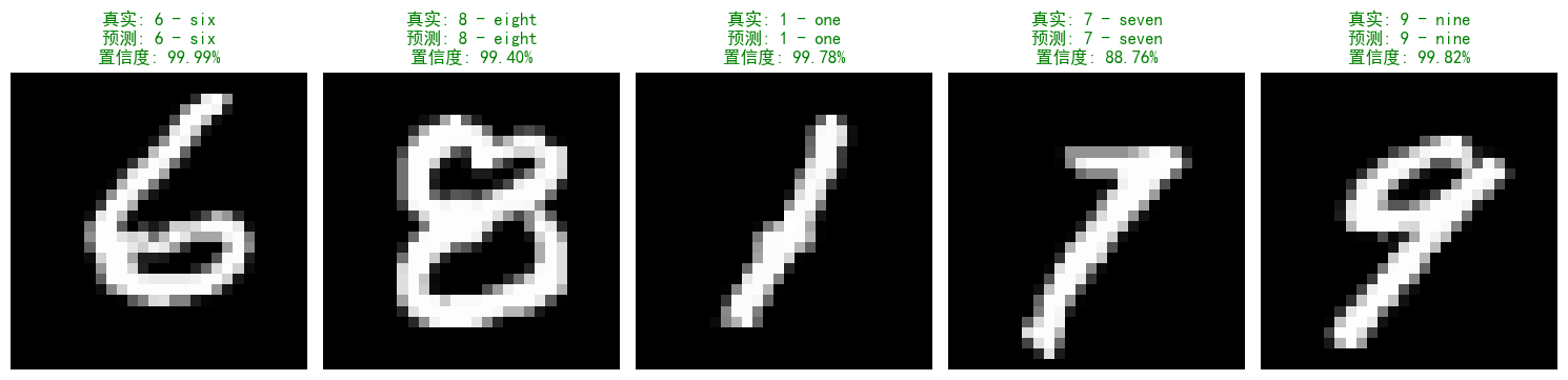
def show_random_predictions(model, test_loader, device, num_images=5):model.eval()# 随机选择索引indices = np.random.choice(len(test_dataset), num_images, replace=False)plt.figure(figsize=(3*num_images, 4))for i, idx in enumerate(indices):# 获取图像和真实标签image, label = test_dataset[idx]image = image.unsqueeze(0).to(device)# 预测并计算概率with torch.no_grad():output = model(image)probs = torch.nn.functional.softmax(output, dim=1)_, predicted = torch.max(output.data, 1)confidence = probs[0][predicted].item()# 转换图像格式image = image.squeeze().cpu().numpy()# 修改为直接取第一个通道(MNIST是单通道)image = image[0] if image.ndim == 3 else image # 处理单通道情况image = image * 0.1307 + 0.3081 # 反归一化# 绘制结果plt.subplot(1, num_images, i+1)plt.imshow(image, cmap='gray') # 明确指定灰度图# 设置标题颜色和内容title_color = 'green' if predicted.item() == label else 'red'title_text = (f'真实: {test_dataset.classes[label]}\n'f'预测: {test_dataset.classes[predicted.item()]}\n'f'置信度: {confidence:.2%}')plt.title(title_text, color=title_color)plt.axis('off')plt.tight_layout()plt.show()# 在训练完成后调用
print("\n随机测试图像预测结果:")
show_random_predictions(model, test_loader, device)开始训练模型...
Epoch: 1/2 | Batch: 100/938 | 单Batch损失: 0.4156 | 累计平均损失: 0.6298
Epoch: 1/2 | Batch: 200/938 | 单Batch损失: 0.2680 | 累计平均损失: 0.4774
Epoch: 1/2 | Batch: 300/938 | 单Batch损失: 0.4445 | 累计平均损失: 0.4096
Epoch: 1/2 | Batch: 400/938 | 单Batch损失: 0.1984 | 累计平均损失: 0.3676
Epoch: 1/2 | Batch: 500/938 | 单Batch损失: 0.3787 | 累计平均损失: 0.3352
Epoch: 1/2 | Batch: 600/938 | 单Batch损失: 0.2049 | 累计平均损失: 0.3130
Epoch: 1/2 | Batch: 700/938 | 单Batch损失: 0.2164 | 累计平均损失: 0.2962
Epoch: 1/2 | Batch: 800/938 | 单Batch损失: 0.1432 | 累计平均损失: 0.2797
Epoch: 1/2 | Batch: 900/938 | 单Batch损失: 0.0901 | 累计平均损失: 0.2655
Epoch 1/2 完成 | 训练准确率: 92.45% | 测试准确率: 96.09%
Epoch: 2/2 | Batch: 100/938 | 单Batch损失: 0.1137 | 累计平均损失: 0.1193
Epoch: 2/2 | Batch: 200/938 | 单Batch损失: 0.2177 | 累计平均损失: 0.1250
Epoch: 2/2 | Batch: 300/938 | 单Batch损失: 0.1939 | 累计平均损失: 0.1253
Epoch: 2/2 | Batch: 400/938 | 单Batch损失: 0.1066 | 累计平均损失: 0.1227
Epoch: 2/2 | Batch: 500/938 | 单Batch损失: 0.0964 | 累计平均损失: 0.1199
Epoch: 2/2 | Batch: 600/938 | 单Batch损失: 0.1582 | 累计平均损失: 0.1185
Epoch: 2/2 | Batch: 700/938 | 单Batch损失: 0.2484 | 累计平均损失: 0.1173
Epoch: 2/2 | Batch: 800/938 | 单Batch损失: 0.1279 | 累计平均损失: 0.1166
Epoch: 2/2 | Batch: 900/938 | 单Batch损失: 0.2397 | 累计平均损失: 0.1163
Epoch 2/2 完成 | 训练准确率: 96.51% | 测试准确率: 96.64%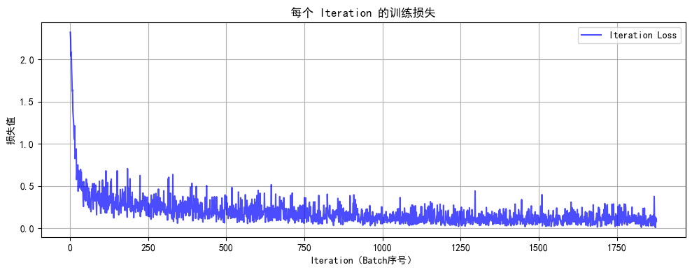
随机测试图像预测结果:
二、彩色图片的规范写法,以CIFAR-10数据集为例
import torch
import torch.nn as nn
import torch.optim as optim
from torchvision import datasets, transforms
from torch.utils.data import DataLoader
import matplotlib.pyplot as plt
import numpy as np# 设置中文字体支持
plt.rcParams["font.family"] = ["SimHei"]
plt.rcParams['axes.unicode_minus'] = False # 解决负号显示问题# 1. 数据预处理
transform = transforms.Compose([transforms.ToTensor(), # 转换为张量transforms.Normalize((0.5, 0.5, 0.5), (0.5, 0.5, 0.5)) # 标准化处理
])# 2. 加载CIFAR-10数据集
train_dataset = datasets.CIFAR10(root='./data',train=True,download=True,transform=transform
)test_dataset = datasets.CIFAR10(root='./data',train=False,transform=transform
)# 3. 创建数据加载器
batch_size = 64
train_loader = DataLoader(train_dataset, batch_size=batch_size, shuffle=True)
test_loader = DataLoader(test_dataset, batch_size=batch_size, shuffle=False)# 4. 定义MLP模型(适应CIFAR-10的输入尺寸)
class MLP(nn.Module):def __init__(self):super(MLP, self).__init__()self.flatten = nn.Flatten() # 将3x32x32的图像展平为3072维向量self.layer1 = nn.Linear(3072, 512) # 第一层:3072个输入,512个神经元self.relu1 = nn.ReLU()self.dropout1 = nn.Dropout(0.2) # 添加Dropout防止过拟合self.layer2 = nn.Linear(512, 256) # 第二层:512个输入,256个神经元self.relu2 = nn.ReLU()self.dropout2 = nn.Dropout(0.2)self.layer3 = nn.Linear(256, 10) # 输出层:10个类别def forward(self, x):# 第一步:将输入图像展平为一维向量x = self.flatten(x) # 输入尺寸: [batch_size, 3, 32, 32] → [batch_size, 3072]# 第一层全连接 + 激活 + Dropoutx = self.layer1(x) # 线性变换: [batch_size, 3072] → [batch_size, 512]x = self.relu1(x) # 应用ReLU激活函数x = self.dropout1(x) # 训练时随机丢弃部分神经元输出# 第二层全连接 + 激活 + Dropoutx = self.layer2(x) # 线性变换: [batch_size, 512] → [batch_size, 256]x = self.relu2(x) # 应用ReLU激活函数x = self.dropout2(x) # 训练时随机丢弃部分神经元输出# 第三层(输出层)全连接x = self.layer3(x) # 线性变换: [batch_size, 256] → [batch_size, 10]return x # 返回未经过Softmax的logits# 检查GPU是否可用
device = torch.device("cuda" if torch.cuda.is_available() else "cpu")# 初始化模型
model = MLP()
model = model.to(device) # 将模型移至GPU(如果可用)criterion = nn.CrossEntropyLoss() # 交叉熵损失函数
optimizer = optim.Adam(model.parameters(), lr=0.001) # Adam优化器# 5. 训练模型(记录每个 iteration 的损失)
def train(model, train_loader, test_loader, criterion, optimizer, device, epochs):model.train() # 设置为训练模式# 记录每个 iteration 的损失all_iter_losses = [] # 存储所有 batch 的损失iter_indices = [] # 存储 iteration 序号for epoch in range(epochs):running_loss = 0.0correct = 0total = 0for batch_idx, (data, target) in enumerate(train_loader):data, target = data.to(device), target.to(device) # 移至GPUoptimizer.zero_grad() # 梯度清零output = model(data) # 前向传播loss = criterion(output, target) # 计算损失loss.backward() # 反向传播optimizer.step() # 更新参数# 记录当前 iteration 的损失iter_loss = loss.item()all_iter_losses.append(iter_loss)iter_indices.append(epoch * len(train_loader) + batch_idx + 1)# 统计准确率和损失running_loss += iter_loss_, predicted = output.max(1)total += target.size(0)correct += predicted.eq(target).sum().item()# 每100个批次打印一次训练信息if (batch_idx + 1) % 100 == 0:print(f'Epoch: {epoch+1}/{epochs} | Batch: {batch_idx+1}/{len(train_loader)} 'f'| 单Batch损失: {iter_loss:.4f} | 累计平均损失: {running_loss/(batch_idx+1):.4f}')# 计算当前epoch的平均训练损失和准确率epoch_train_loss = running_loss / len(train_loader)epoch_train_acc = 100. * correct / total# 测试阶段model.eval() # 设置为评估模式test_loss = 0correct_test = 0total_test = 0with torch.no_grad():for data, target in test_loader:data, target = data.to(device), target.to(device)output = model(data)test_loss += criterion(output, target).item()_, predicted = output.max(1)total_test += target.size(0)correct_test += predicted.eq(target).sum().item()epoch_test_loss = test_loss / len(test_loader)epoch_test_acc = 100. * correct_test / total_testprint(f'Epoch {epoch+1}/{epochs} 完成 | 训练准确率: {epoch_train_acc:.2f}% | 测试准确率: {epoch_test_acc:.2f}%')# 绘制所有 iteration 的损失曲线plot_iter_losses(all_iter_losses, iter_indices)return epoch_test_acc # 返回最终测试准确率# 6. 绘制每个 iteration 的损失曲线
def plot_iter_losses(losses, indices):plt.figure(figsize=(10, 4))plt.plot(indices, losses, 'b-', alpha=0.7, label='Iteration Loss')plt.xlabel('Iteration(Batch序号)')plt.ylabel('损失值')plt.title('每个 Iteration 的训练损失')plt.legend()plt.grid(True)plt.tight_layout()plt.show()# 7. 执行训练和测试
epochs = 20 # 增加训练轮次以获得更好效果
print("开始训练模型...")
final_accuracy = train(model, train_loader, test_loader, criterion, optimizer, device, epochs)
print(f"训练完成!最终测试准确率: {final_accuracy:.2f}%")# 8. 随机选择测试图像进行预测展示
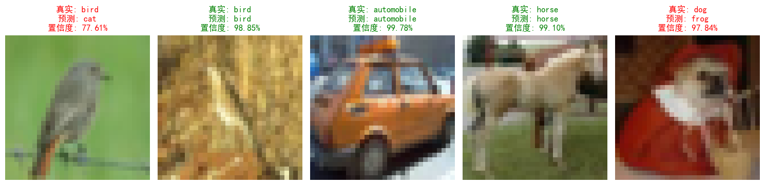
def show_random_predictions(model, test_loader, device, num_images=5):model.eval()# 随机选择索引indices = np.random.choice(len(test_dataset), num_images, replace=False)plt.figure(figsize=(3*num_images, 4))for i, idx in enumerate(indices):# 获取图像和真实标签image, label = test_dataset[idx]image = image.unsqueeze(0).to(device)# 预测并计算概率with torch.no_grad():output = model(image)probs = torch.nn.functional.softmax(output, dim=1)_, predicted = torch.max(output.data, 1)confidence = probs[0][predicted].item()# 转换图像格式(CIFAR-10专用)image = image.squeeze().cpu().numpy()image = np.transpose(image, (1, 2, 0)) # 从(C,H,W)转为(H,W,C)image = image * 0.5 + 0.5 # 反归一化# 绘制结果(CIFAR-10不需要cmap='gray')plt.subplot(1, num_images, i+1)plt.imshow(image) # 设置标题颜色和内容title_color = 'green' if predicted.item() == label else 'red'title_text = (f'真实: {test_dataset.classes[label]}\n'f'预测: {test_dataset.classes[predicted.item()]}\n'f'置信度: {confidence:.2%}')plt.title(title_text, color=title_color)plt.axis('off')plt.tight_layout()plt.show()# 在训练完成后调用
print("\n随机测试图像预测结果:")
show_random_predictions(model, test_loader, device)开始训练模型...
Epoch: 1/20 | Batch: 100/782 | 单Batch损失: 1.8490 | 累计平均损失: 1.9064
Epoch: 1/20 | Batch: 200/782 | 单Batch损失: 1.9917 | 累计平均损失: 1.8319
Epoch: 1/20 | Batch: 300/782 | 单Batch损失: 1.6255 | 累计平均损失: 1.7918
Epoch: 1/20 | Batch: 400/782 | 单Batch损失: 1.4693 | 累计平均损失: 1.7604
Epoch: 1/20 | Batch: 500/782 | 单Batch损失: 1.8785 | 累计平均损失: 1.7441
Epoch: 1/20 | Batch: 600/782 | 单Batch损失: 1.5239 | 累计平均损失: 1.7261
Epoch: 1/20 | Batch: 700/782 | 单Batch损失: 1.5979 | 累计平均损失: 1.7132
Epoch 1/20 完成 | 训练准确率: 39.59% | 测试准确率: 45.31%
Epoch: 2/20 | Batch: 100/782 | 单Batch损失: 1.3397 | 累计平均损失: 1.4856
Epoch: 2/20 | Batch: 200/782 | 单Batch损失: 1.4475 | 累计平均损失: 1.4658
Epoch: 2/20 | Batch: 300/782 | 单Batch损失: 1.3311 | 累计平均损失: 1.4698
Epoch: 2/20 | Batch: 400/782 | 单Batch损失: 1.5560 | 累计平均损失: 1.4726
Epoch: 2/20 | Batch: 500/782 | 单Batch损失: 1.3987 | 累计平均损失: 1.4686
Epoch: 2/20 | Batch: 600/782 | 单Batch损失: 1.4540 | 累计平均损失: 1.4664
Epoch: 2/20 | Batch: 700/782 | 单Batch损失: 1.3138 | 累计平均损失: 1.4620
Epoch 2/20 完成 | 训练准确率: 48.36% | 测试准确率: 50.02%
Epoch: 3/20 | Batch: 100/782 | 单Batch损失: 1.3247 | 累计平均损失: 1.3399
Epoch: 3/20 | Batch: 200/782 | 单Batch损失: 1.5797 | 累计平均损失: 1.3359
Epoch: 3/20 | Batch: 300/782 | 单Batch损失: 1.7371 | 累计平均损失: 1.3417
Epoch: 3/20 | Batch: 400/782 | 单Batch损失: 1.2458 | 累计平均损失: 1.3385
Epoch: 3/20 | Batch: 500/782 | 单Batch损失: 1.3252 | 累计平均损失: 1.3355
Epoch: 3/20 | Batch: 600/782 | 单Batch损失: 1.2957 | 累计平均损失: 1.3373
Epoch: 3/20 | Batch: 700/782 | 单Batch损失: 1.3832 | 累计平均损失: 1.3398
...
Epoch: 20/20 | Batch: 500/782 | 单Batch损失: 0.6388 | 累计平均损失: 0.3730
Epoch: 20/20 | Batch: 600/782 | 单Batch损失: 0.3712 | 累计平均损失: 0.3795
Epoch: 20/20 | Batch: 700/782 | 单Batch损失: 0.3770 | 累计平均损失: 0.3884
Epoch 20/20 完成 | 训练准确率: 86.10% | 测试准确率: 53.29%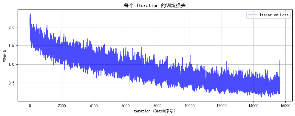
随机测试图像预测结果:
![题海拾贝:P8598 [蓝桥杯 2013 省 AB] 错误票据](https://i-blog.csdnimg.cn/direct/6848721f37aa40ca84322a78517857ab.png)