定义

三级淋巴结构 （TLS，Tumor Lymphoid Structure）：是指在非淋巴组织中的慢性炎症部位（包括癌症）形成的异位淋巴细胞聚集体。

目前，分割和量化 TLS 的金标准是基于对 T（CD3: 用于标记T细胞） 和 B 淋巴细胞（CD20: 用于标记B细胞）使用多重免疫组织化学 （mIHC） 染色的病理特征。

临床意义

尽管肿瘤微环境中淋巴组织样结构（TLS）形成的确切机制尚未完全明确，但已有研究显示TLS与多种癌症类型的积极免疫治疗反应及改善的临床预后密切相关。因此，肿瘤病灶中TLS的存在可以作为预测患者临床预后和对免疫检查点阻断（ICB）治疗反应的重要指标。

淋巴浸润细胞是 TME 的常见成分（同时巨噬细胞通常也是肿瘤微环境中最为丰富的免疫细胞类型之一），大多数免疫细胞可以在肿瘤的中心区域或边缘区域以不同的比例被发现。因此，可以结合免疫微环境进一步分析。

文献证明TLS指导预后和免疫治疗反应

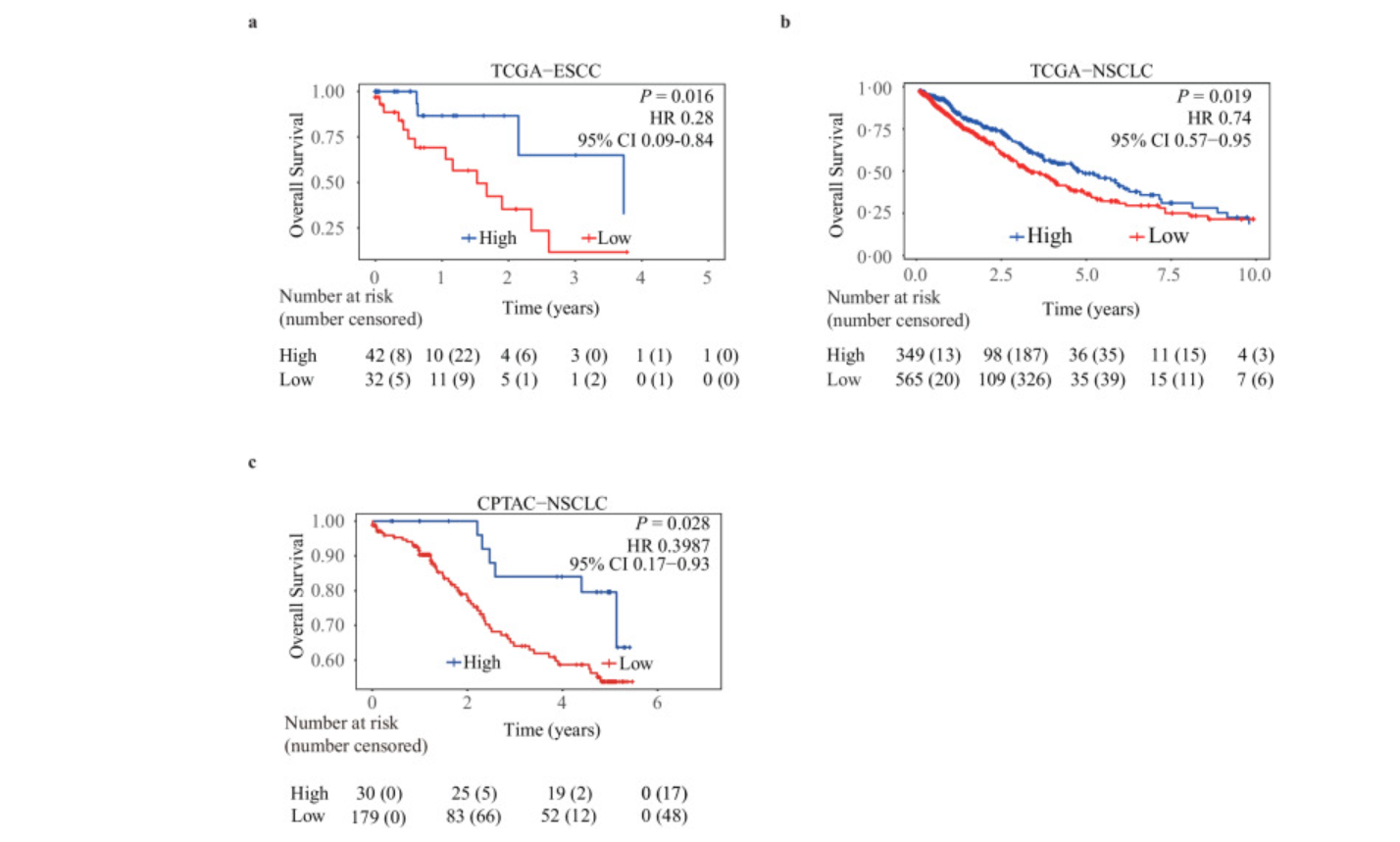
- 指导预后

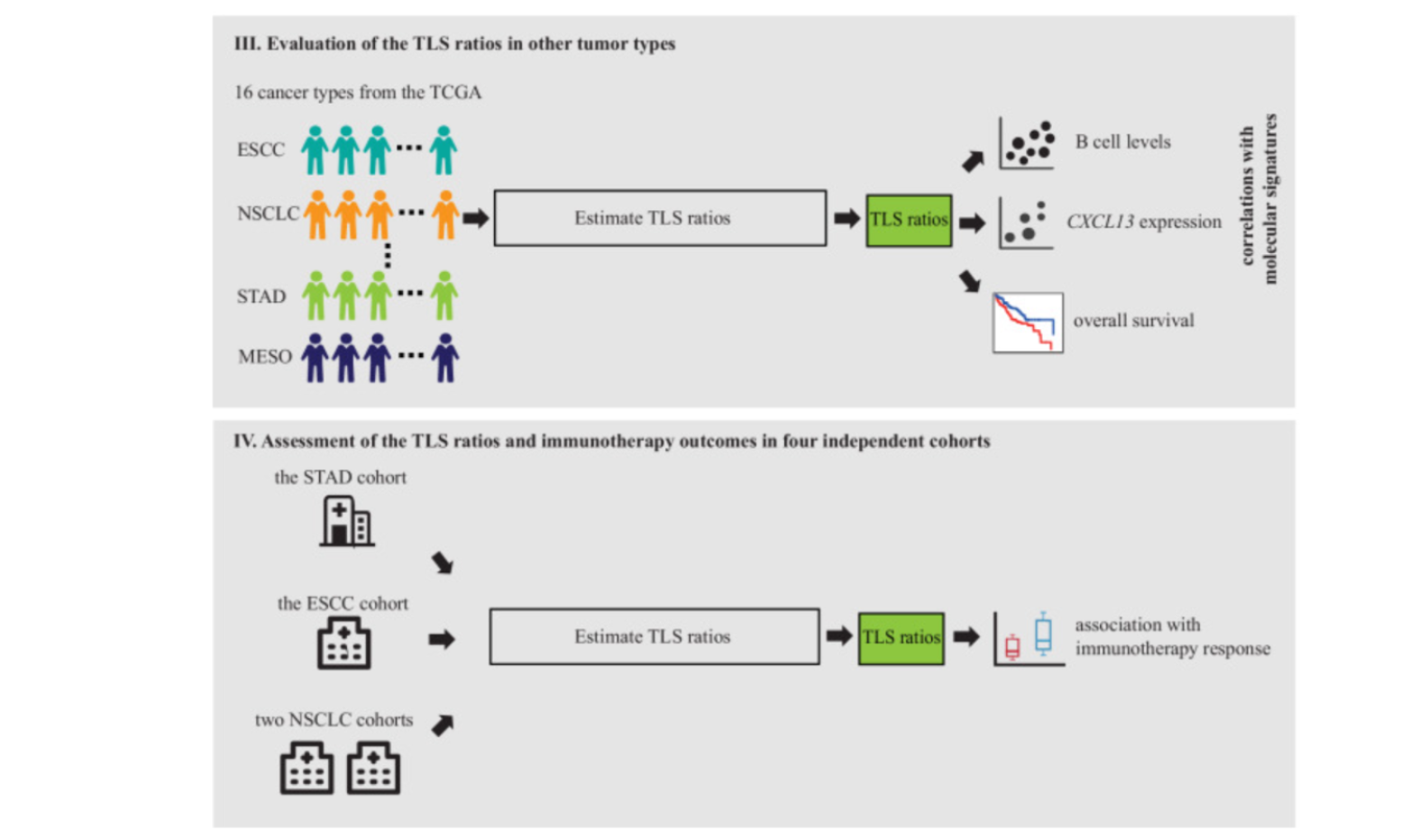
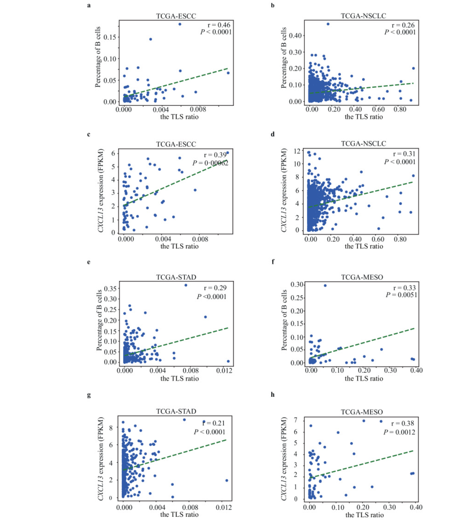
- 指导免疫治疗响应：估计的 TLS 比率与各种 TCGA 肿瘤类型的 B 淋巴细胞水平和 CXCL13 表达相关分析

CXCL13 是一种与 TLS 形成相关的趋化因子。CXCL13的表达增加通常促进B细胞和Tfh细胞在炎症部位的聚集。

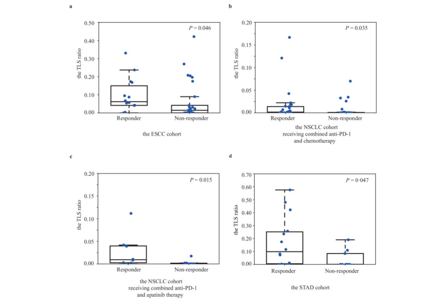
- 指导免疫治疗响应：四个独立队列的 TLS 比率和免疫治疗结果进一步验证验证

基于深度学习预测TLS比例的方法：

本文近似TLS ratio 计算方法为：TLS 比率=预测的TLS面积/病理组织面积。

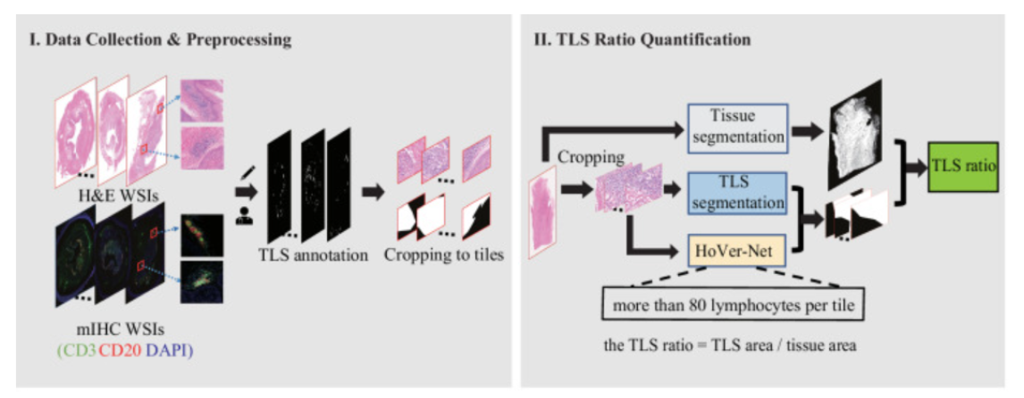
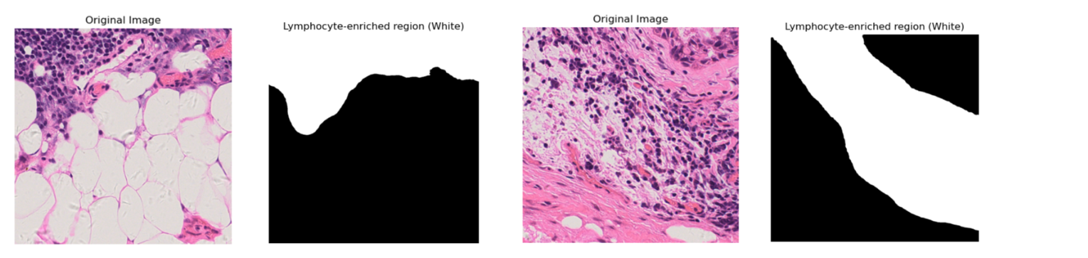
具体实现存在三个分支：（1）直接分割HE上的组织面积（OpenCV Python 包中的 OTSU 方法）；（2）将HE切割成大小为1024或512的patch，采用HE 作为原图，mIHC作为TLS鉴定的金标准。构建TLS预测模型，输出为patch对应的黑白图，白色为TLS区域，黑色为组织区域。（3）采用hovernet保证每张patch上的淋巴细胞数量不低于80。最后将鉴定包括TLS区域的patch上的白色区域面积相加作为TLS面积。

具体代码实现 TLS ratio计算：

Step0：先修改一下get_slide_tls.py

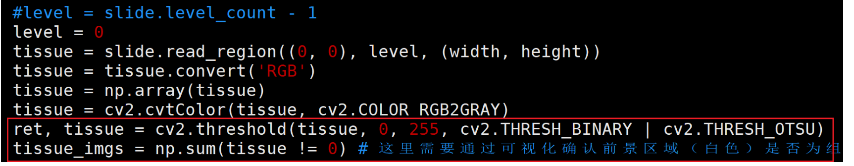
• 组织区域面积计算用的是最小分辨率，但patch分割是在level 0 ，代码为patch = slide.read_region((int(j * ExtractSize * (1 - RepetitionRate)), int(i * ExtractSize * (1 - RepetitionRate))), 0, (ExtractSize, ExtractSize))，因此，将level同样设置为0。

• 这句代码用于分割组织区域和背景区域(默认组织块比背景块亮，组织块为白色，现实并不是如此)。因此，这里需要通过可视化（代码如下）确认前景区域（白色）是否为组织区域，若不是，则可以通过cv2.THRESH_BINARY_INV来实现或者直接计算像素点不为255的面积。
  

import cv2
import numpy as np
import matplotlib.pyplot as plt
from PIL import Image
import openslide# 打开病理切片图像
ref_img_path = "./slide/TCGA-4C-A93U-01Z-00-DX2.15B0C115-43F2-415E-AB24-315635E655AA.svs"
slide = openslide.OpenSlide(ref_img_path)# 获取图像的宽度和高度
width, height = slide.dimensions
print(width, height,width*height)# 选择最低分辨率级别
level = 0 #slide.level_count - 3# 从最低分辨率级别读取整个图像
tissue = slide.read_region((0, 0), level, (width, height))# 转换为RGB格式
tissue = tissue.convert('RGB')# 转换为NumPy数组
tissue = np.array(tissue)# 转换为灰度图像
tissue_gray = cv2.cvtColor(tissue, cv2.COLOR_RGB2GRAY)# 在图像处理中，将白色（值为255）视为前景，而将黑色（值为0）视为背景，这主要是基于一种约定俗成的视觉习惯和处理逻辑。
# 使用Otsu阈值化方法进行分割，cv2.THRESH_BINARY：将像素值大于阈值的像素设置为最大值（255），小于或等于阈值的像素设置为 0。
ret, tissue_thresh = cv2.threshold(tissue_gray, 0, 255, cv2.THRESH_BINARY | cv2.THRESH_OTSU) # 使用matplotlib显示分割后的图像
plt.figure(figsize=(12, 6))# 显示原始图像
plt.subplot(1, 2, 1)
plt.title("Original Image")
plt.imshow(tissue)
plt.axis('off')# 显示分割后的图像
plt.subplot(1, 2, 2)
plt.title("Segmented Image (Otsu Thresholding)")
plt.imshow(tissue_thresh, cmap='gray')
plt.axis('off')plt.show()

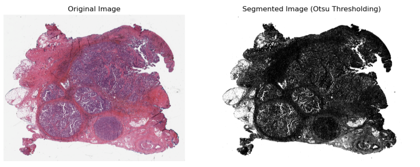
# 方法一：反转颜色，大于阈值的设置为黑色，小于阈值的设置为白色
ret, tissue_thresh = cv2.threshold(tissue_gray, 0, 255, cv2.THRESH_BINARYN_INV | cv2.THRESH_OTSU) 
tissue_pixels = np.sum(tissue_thresh != 0) 
print("组织的像素点数量为：",tissue_pixels)# 方法二：直接计算黑色区域的像素点个数（面积）
ret, tissue_thresh = cv2.threshold(tissue_gray, 0, 255, cv2.THRESH_BINARY | cv2.THRESH_OTSU) 
tissue_pixels = np.sum(tissue_thresh != 255) 
print("组织的像素点数量为：",tissue_pixels)

Step1：切割病理切片为patch并分割patch上的淋巴结富集区域

#### 切割病理切片为patch并分割patch上的淋巴结富集区域 ###
# 输入目录：HNSC，放置原始病理切片文件（.ndpi或.svs）
# 输出目录1：predictions，每个切片会生成一个目录，目录下包含images（patch），lyms（基于hovernet识别的淋巴细胞）和masks（淋巴细胞富集区域）三个子目录。保存在上述子目录中的patch需要满足一定筛选标准（1.淋巴细胞数量大于或等于这个阈值（80）；2. 非零像素比例大于10%，小于10%即认为该图像块主要是背景或空白区域）。
# 输出目录2：predictions/tissue_predictions/目录中的.txt文件记录了每个病理切片图像的组织区域大小，这个大小是通过计算组织掩码中非零像素的数量得到的，反映了整张病理切片图像上组织区域的面积。python get_slide_tls.py --cancer_type HNSC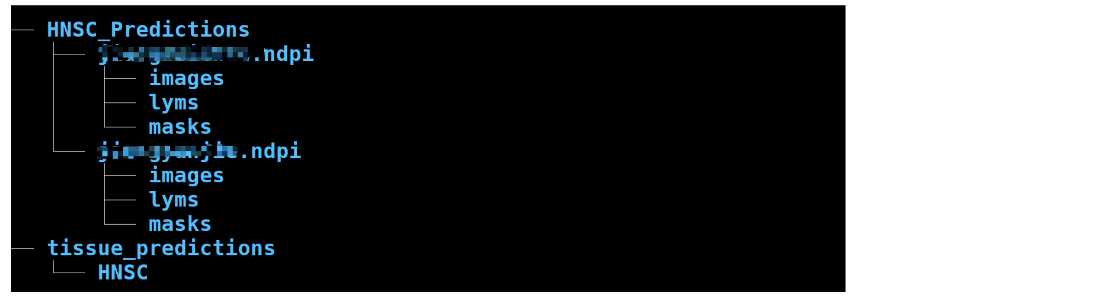

Step2：统计病理组织面积为dataframe

result_dir = "./predictions/tissue_predictions/HNSC//"
df_tissue_area = pd.DataFrame(columns=["slide_id","tissue_area_slide_level"])
for tis_area_file in os.listdir(result_dir):tis_area_file = os.path.join(result_dir,tis_area_file)tmp_df = pd.read_csv(tis_area_file,sep="\t",header=None,names=["slide_id","tissue_area_slide_level"])df_tissue_area = pd.concat([df_tissue_area,tmp_df])
df_tissue_area.tissue_area_slide_level = df_tissue_area.tissue_area_slide_level.astype("float")
df_tissue_area

Step3：计算淋巴富集区域面积

def lyms_area_calculation(png_path,show = False):import cv2import numpy as npimport matplotlib.pyplot as plt# 读取图像image = cv2.imread(png_path, cv2.IMREAD_GRAYSCALE)# 应用Otsu阈值分割ret, thresh = cv2.threshold(image, 0, 255, cv2.THRESH_OTSU)# 计算白色区域的面积# 首先找到白色区域的轮廓contours, _ = cv2.findContours(thresh, cv2.RETR_EXTERNAL, cv2.CHAIN_APPROX_SIMPLE)# 计算面积area = 0for contour in contours:area += cv2.contourArea(contour)print(f'Area of white region: {area}') #, Area of whole patch: {1024*1024})if show == True:# 显示原图和分割后的图plt.figure(figsize=(10, 5))plt.subplot(1, 2, 1)plt.title('Original Image')plt.imshow(image, cmap='gray')plt.axis('off')plt.subplot(1, 2, 2)plt.title('Otsu Thresholding')plt.imshow(thresh, cmap='gray')plt.axis('off')plt.show()return arearesult_dir = "./predictions/HNSC_Predictions/"
df_lym_area = pd.DataFrame(columns=["slide_id","patch_id","lyms_area"])for svs in tqdm(os.listdir(result_dir)):print(svs)## 计算淋巴细胞富集区域面积（白色区域面积）tis_path = os.path.join(result_dir,svs,"masks")for png_path in tqdm(os.listdir(tis_path)):png_path_ = os.path.join(tis_path,png_path)print(png_path_)lyms_area = lyms_area_calculation(png_path_,show = False)df_lym_area.loc[len(df_lym_area)] = [svs,png_path,lyms_area]
df_lym_area_slide = df_lym_area.groupby("slide_id").agg("sum").reset_index()
df_lym_area_slide.columns = ["slide_id","lyms_area_slide_level"]
df_lym_area = pd.merge(df_lym_area,df_lym_area_slide,how="left",on="slide_id")
df_lym_area.to_csv("slide_lyms_area.csv",index=False)
df_lym_area.head()

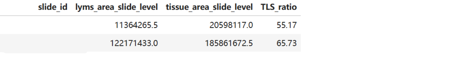
Step4：TLS ratio计算

TLS =  pd.merge(df_lym_area,df_tissue_area,how="inner",on=["slide_id"])
TLS = TLS[["slide_id","lyms_area_slide_level","tissue_area_slide_level"]].drop_duplicates()
TLS["TLS_ratio"] = round(TLS["lyms_area_slide_level"]/TLS["tissue_area_slide_level"]*100,2)
TLS

Reference

文献：

Deep learning on tertiary lymphoid structures in hematoxylin-eosin predicts cancer prognosis and immunotherapy responsehttps://github.com/zonechen1994/AI_TLS_segmentation

Tertiary lymphoid structures are critical for cancer prognosis and therapeutic response

代码：

GitHub - zonechen1994/AI_TLS_segmentation