PINN for PDE(偏微分方程)3 - 正向问题 - Burgers’ equation
目录
- PINN for PDE(偏微分方程)3 - 正向问题 - Burgers’ equation
- 一、什么是PINN的正问题
- 二、求解的实际例子 - Burgers’ equation
- 2.1 Burgers方程
- 2.2 无解析解解决办法 - 龙哥库达(Runge-Kutta 4th Order Method, RK4)
- 三、基于Pytorch实现的代码 - 分解
- 3.1 longge.py 文件
- 3.2 main.py 文件
- 3.2.1 引入库函数
- 3.2.2 设置超参数
- 3.2.3 设计随机种子,确保复现结果的一致性
- 3.2.4 对于条件等式生成对应的训练数据
- 3.2.5 定义PINN网络
- 3.2.6 定义求导函数
- 3.2.7 定义损失函数
- 3.2.8 模型训练
- 3.2.9 绘制结果图像
- 结果图
- 4.1 真实结果图
- 4.2 PINN预测结果图
- 4.3 两者误差图
- 参考
一、什么是PINN的正问题
在 PINN(Physics-Informed Neural Networks,物理信息神经网络)中,**正问题(Forward Problem)**指的是:
给定一个偏微分方程(PDE)的形式、边界条件和初始条件,求解该方程在定义域内的解函数。
在 PINN 框架下,求解正问题的基本步骤如下:
- 构建神经网络 u θ ( x , t ) u_\theta(x, t) uθ(x,t) 作为 PDE 解的近似;
- 利用自动微分计算偏导数,将 PDE 表达为损失函数项;
- 同时将边界条件和初始条件也转化为损失函数;
- 通过最小化总损失来训练神经网络参数 θ \theta θ,使其近似满足物理规律。
正问题的特征是:问题的数学描述是充分确定的,即 PDE 与条件信息足够多,因此目标是通过神经网络来模拟已知物理过程。
二、求解的实际例子 - Burgers’ equation
2.1 Burgers方程
Burgers方程的定义为:
∂ u ∂ t + u ∂ u ∂ x = v ∂ 2 u ∂ x 2 , x ∈ [ − 1 , 1 ] , t ∈ [ 0 , 1 ] , u ( x , 0 ) = − sin ( π x ) , u ( − 1 , t ) = u ( 1 , t ) = 0 , \begin{array}{l} \frac{\partial u}{\partial t}+u\frac{\partial u}{\partial x}=v\frac{\partial ^2u}{\partial x^2},\quad x\in [-1,1],t\in [0,1],\\ u(x,0)=-\sin\mathrm{(}\pi x),\\ u(-1,t)=u(1,t)=0,\\ \end{array} ∂t∂u+u∂x∂u=v∂x2∂2u,x∈[−1,1],t∈[0,1],u(x,0)=−sin(πx),u(−1,t)=u(1,t)=0,
其中,u 为流速,ν 为流体的粘度。在本文中,ν 设为 0.01 / π。
2.2 无解析解解决办法 - 龙哥库达(Runge-Kutta 4th Order Method, RK4)
由于 Burgers 方程的解析解比较的复杂,并且没有显式解析解(好像看了一下是带积分的),因此本文主要采用的方法是利用4阶的龙哥库达方法进行数值求解,从而构造训练数据集。四阶龙格-库塔方法(RK4)是一种用于常微分方程初值问题(IVP)的数值求解方法,具有较高的精度与稳定性,是工程与科学计算中最常用的数值积分方法之一。
一、问题背景
考虑一个初值问题形式如下的常微分方程(ODE):
d y d t = f ( t , y ) , y ( t 0 ) = y 0 \frac{dy}{dt} = f(t, y), \quad y(t_0) = y_0 dtdy=f(t,y),y(t0)=y0
我们希望在某个时间区间内,求出 y ( t ) y(t) y(t) 的数值解。
RK4 方法通过在当前点 t n t_n tn 处对斜率的多次采样来估计下一步的解 y n + 1 y_{n+1} yn+1,实现高阶精度。
二、RK4 方法公式
设步长为 h h h,则 RK4 的迭代格式如下:
k 1 = f ( t n , y n ) k 2 = f ( t n + h 2 , y n + h 2 k 1 ) k 3 = f ( t n + h 2 , y n + h 2 k 2 ) k 4 = f ( t n + h , y n + h k 3 ) y n + 1 = y n + h 6 ( k 1 + 2 k 2 + 2 k 3 + k 4 ) \begin{aligned} k_1 &= f(t_n, y_n) \\ k_2 &= f\left(t_n + \frac{h}{2},\ y_n + \frac{h}{2}k_1\right) \\ k_3 &= f\left(t_n + \frac{h}{2},\ y_n + \frac{h}{2}k_2\right) \\ k_4 &= f\left(t_n + h,\ y_n + hk_3\right) \\ y_{n+1} &= y_n + \frac{h}{6}(k_1 + 2k_2 + 2k_3 + k_4) \end{aligned} k1k2k3k4yn+1=f(tn,yn)=f(tn+2h, yn+2hk1)=f(tn+2h, yn+2hk2)=f(tn+h, yn+hk3)=yn+6h(k1+2k2+2k3+k4)
其中:
- k 1 k_1 k1 是在区间起点的斜率;
- k 2 k_2 k2 和 k 3 k_3 k3 是中点的斜率(通过预测点计算);
- k 4 k_4 k4 是终点的斜率;
- y n + 1 y_{n+1} yn+1 是在 t n + 1 = t n + h t_{n+1} = t_n + h tn+1=tn+h 处的近似解。
该方法综合了多个点的斜率估计,以提升准确性,局部截断误差为 O ( h 5 ) O(h^5) O(h5),整体误差为 O ( h 4 ) O(h^4) O(h4)。
三、算法步骤总结
- 给定初始条件: t 0 t_0 t0, y 0 y_0 y0,以及步长 h h h;
- 对于每个时间点:
- 计算 k 1 k_1 k1 到 k 4 k_4 k4;
- 更新解 y n + 1 y_{n+1} yn+1;
- 更新时间 t n + 1 = t n + h t_{n+1} = t_n + h tn+1=tn+h;
- 重复直到达到目标时间。
四、RK4 与其他方法对比
| 方法 | 局部误差阶 | 全局误差阶 | 是否显式 | 备注 |
|---|---|---|---|---|
| 欧拉法 | O ( h 2 ) O(h^2) O(h2) | O ( h ) O(h) O(h) | 是 | 简单但不精确 |
| 改进欧拉 | O ( h 3 ) O(h^3) O(h3) | O ( h 2 ) O(h^2) O(h2) | 是 | 使用中点斜率 |
| RK4 | O ( h 5 ) O(h^5) O(h5) | O ( h 4 ) O(h^4) O(h4) | 是 | 精度与效率兼顾 |
| 隐式方法 | 可变 | 可变 | 否 | 适合刚性问题 |
三、基于Pytorch实现的代码 - 分解
3.1 longge.py 文件
- 4阶龙格库达实现Burgers方程我直接用的现成的CSDN上的代码,该代码出处已标注在下面,本文仅对其进行了简单修改,提取出结果进行PINN数据备用。
""" Solving the Burgers' Equation using a 4th order Runge-Kutta method """import numpy as np
import matplotlib.pyplot as plt
from mpl_toolkits.mplot3d import Axes3D  # 添加在顶部 import 部分
from matplotlib import cmdef rk4(f, u, t, dx, h):"""Fourth-order Runge-Kutta method for computing u at the next time step."""k1 = f(u, t, dx)k2 = f(u + 0.5*h*k1, t + 0.5*h, dx)k3 = f(u + 0.5*h*k2, t + 0.5*h, dx)k4 = f(u + h*k3, t + h, dx)return u + (h/6)*(k1 + 2*k2 + 2*k3 + k4)def dudx(u, dx):"""Approximate the first derivative using the centered finite differenceformula."""first_deriv = np.zeros_like(u)# wrap to compute derivative at endpointsfirst_deriv[0] = (u[1] - u[-1]) / (2*dx)first_deriv[-1] = (u[0] - u[-2]) / (2*dx)# compute du/dx for all the other pointsfirst_deriv[1:-1] = (u[2:] - u[0:-2]) / (2*dx)return first_derivdef d2udx2(u, dx):"""Approximate the second derivative using the centered finite differenceformula."""second_deriv = np.zeros_like(u)  # 创建一个新数组second_deriv,其形状和类型与给定数组u相同,但是所有元素都被设置为 0。# wrap to compute second derivative at endpointssecond_deriv[0] = (u[1] - 2*u[0] + u[-1]) / (dx**2)second_deriv[-1] = (u[0] - 2*u[-1] + u[-2]) / (dx**2)# compute d2u/dx2 for all the other pointssecond_deriv[1:-1] = (u[2:] - 2*u[1:-1] + u[0:-2]) / (dx**2)return second_derivdef f(u, t, dx, nu=0.01/np.pi):return -u*dudx(u, dx) + nu*d2udx2(u, dx)def make_square_axis(ax):ax.set_aspect(1 / ax.get_data_ratio())def burgers(x0, xN, N, t0, tK, K):x = np.linspace(x0, xN, N)  # evenly spaced spatial pointsdx = (xN - x0) / float(N - 1)  # space between each spatial pointdt = (tK - t0) / float(K)  # space between each temporal pointh = 2e-6  # time step for runge-kutta methodu = np.zeros(shape=(K, N))# u[0, :] = 1 + 0.5*np.exp(-(x**2))  # compute u at initial time stepu[0, :] = -np.sin(np.pi*x)for idx in range(K-1):  # for each temporal point perform runge-kutta methodti = t0 + dt*idxU = u[idx, :]for step in range(1000):t = ti + h*stepU = rk4(f, U, t, dx, h)u[idx+1, :] = UX, T = np.meshgrid(np.linspace(x0, xN, N), np.linspace(t0, tK, K))return X,T,u# X,T,u = burgers(-10, 10, 1024, 0, 50, 500)
x0, xN, N, t0, tK, K = -1, 1, 512, 0, 1, 500X,T,Z = burgers(x0, xN, N, t0, tK, K)if __name__ == '__main__':# # 二维绘制热力图# plt.imshow(u, extent=[x0, xN, t0, tK])# plt.imshow(u.T, interpolation='nearest', cmap='rainbow',#            extent=[t0, tK, x0, xN], origin='lower', aspect='auto')# plt.xlabel('t')# plt.ylabel('x')# plt.colorbar()# plt.show()# 绘制三维曲面图fig = plt.figure()ax = Axes3D(fig)fig.add_axes(ax)ax.plot_surface(X, T, Z)ax.text2D(0.5, 0.9, "burgers_longge", transform=ax.transAxes)plt.show()fig.savefig("result_img/burgers.png")
3.2 main.py 文件
3.2.1 引入库函数
import torch
import matplotlib.pyplot as plt
from mpl_toolkits.mplot3d import Axes3D
import osfrom longge import X,T,Z # 利用龙格库塔方法求解的 Burgers 数值解
3.2.2 设置超参数
# ====================== 超参数 ======================
epochs = 10000         # 训练轮数
h = 100               # 作图时的网格密度
N = 1000              # PDE残差点(训练内点)
N1 = 100            # 边界条件点
N2 = 1000             # 数据点(已知解)device=torch.device('cuda' if torch.cuda.is_available() else 'cpu')
3.2.3 设计随机种子,确保复现结果的一致性
def setup_seed(seed):torch.manual_seed(seed)  # 设置 PyTorch 中 CPU 上的随机数种子,使得所有如 torch.rand()、torch.randn() 等函数在 CPU 上的随机数生成具有可重复性。torch.cuda.manual_seed_all(seed) # 设置所有 GPU 设备上的随机数种子。GPU 上也有自己的随机数生成器,用于模型参数初始化、Dropout 等操作。torch.backends.cudnn.deterministic = True # 设置 cuDNN 后端为确定性模式。'''cuDNN 是 NVIDIA 为深度学习优化的加速库,但它为了加速有时使用了非确定性算法(比如卷积时自动选择最快的实现方式,某些可能会导致浮点计算顺序不同)。这个设置会强制它只使用确定性算法(牺牲一些速度),确保每次前向/反向传播都一致。'''# 设置随机数种子
setup_seed(888888)
3.2.4 对于条件等式生成对应的训练数据
# Domain and Sampling,内点采样,这里的Burgers的输入是x和t,输出的是u
def interior(n=N):# 生成 PDE(偏微分方程)区域内的训练点# 随机生成 n 个 x 坐标(范围在 [-1, 1)),所以只需要把[0,1) (torch.rand():生成 0 到 1 之间的均匀分布) 的数据调整下就行x = (torch.rand(n, 1)*2-1) .to(device)# 随机生成 n 个 t 坐标(范围在 [0, 1))t = torch.rand(n, 1).to(device)# 计算对应点的“条件值”(可能是解析解、真值或用于损失函数的目标值)# 这里定义为 cond = 0,# 是里面的点偏导等于的一个值# 注意,这里的*因为都是(n,1)的大小的数据,因此,*号都是用于逐个相乘,最终也是得到了(n,1)的数据,如果是矩阵可能会需要torch.matmulcond = torch.zeros_like(t).to(device)# 返回的 x 和 y 启用自动求导功能,以便后续可用于计算梯度(如 PDE 中的导数)return x.requires_grad_(True), t.requires_grad_(True), cond# 边界条件的第一个,对u(x,0)等于sin(pi*x)
def down_1(n=N1):# 下边界上的 u(x, 0) = - sin(pi*x) 条件# 随机生成 n 个 x 坐标,范围在 [-1, 1)x = (torch.rand(n, 1)*2-1) .to(device)t = torch.zeros_like(x).to(device)# 条件值:下边界上的 u(x, 0) = sin(pi*x) 条件,即函数在边界上的值等于 sin(pi*x)cond = - torch.sin(torch.pi*x)# 返回启用自动求导的 x、y,以及边界条件值 condreturn x.requires_grad_(True), t.requires_grad_(True), cond# 这个是边界条件的第二个,对u(-1,t)=0
def down_2(n=N1):# 边界 u(-1,t)=0t = torch.rand(n, 1).to(device)x = -torch.ones_like(t).to(device) # 全设置为-1# print(x[0])cond = torch.zeros_like(t).to(device)return x.requires_grad_(True), t.requires_grad_(True), cond# 这个是边界条件的第三个,对u(1,t)=0
def down_3(n=N1):# 边界 u(1,t)=0t = torch.rand(n, 1).to(device)x = torch.ones_like(t).to(device) # 全设置为1cond = torch.zeros_like(t).to(device)return x.requires_grad_(True), t.requires_grad_(True), cond'''
# 到这里为止,都是在构建数据集,对每个微分方程(包括边界点和中间点)都构建对应的数据集,包含(x,y,对应的条件值(微分方程的真值部分))
''''''
# 真实数据模拟
'''# 到这里Burger的解析解不知道。所以用数值解来作为真实数据。
# 真实解的数据点(监督学习),也就是构建真实数据,这里采用的是数值解def data_interior(n=N2):# 内点t = torch.tensor(T, dtype=torch.float32, device=device).reshape(-1, 1)x = torch.tensor(X, dtype=torch.float32, device=device).reshape(-1, 1)cond = torch.tensor(Z, dtype=torch.float32, device=device).reshape(-1, 1)return x.requires_grad_(True), t.requires_grad_(True), cond
'''
# 因此综合来说,解决一个PINN的正向问题,需要对应的真实数据,(输入(x,y),输出(value)),边界条件的数据,(x_边界,y_边界,value_边界条件)
# 训练的时候,输入网络输入信息(比如位置或者时间信息等等),输出为值,此时计算其数据loss,
如果是边界的位置上,需要计算其边界loss(因为正常来说,我们能拿到的数据都是中间的那些真实数据,我们都需要手动去构建边界的数据去使其满足边界条件)。
'''
3.2.5 定义PINN网络
# Neural Network,简单的一个的神经网络。
class MLP(torch.nn.Module):def __init__(self):super(MLP, self).__init__()# 这里仍然是两个输入,一个是时间t一个是x,输出的话是uself.net = torch.nn.Sequential(torch.nn.Linear(2, 32),torch.nn.Tanh(),torch.nn.Linear(32, 32),torch.nn.Tanh(),torch.nn.Linear(32, 32),torch.nn.Tanh(),torch.nn.Linear(32, 32),torch.nn.Tanh(),torch.nn.Linear(32, 1))def forward(self, x):return self.net(x)# MSEloss,其实就是平方损失,L2距离
# Loss
loss = torch.nn.MSELoss()
3.2.6 定义求导函数
# 这个是单纯是用于求导,因此不需要改变里面的变量
def gradients(u, x, order=1):"""计算函数 u 对变量 x 的高阶导数。参数:u (torch.Tensor): 待求导的函数输出。x (torch.Tensor): 自变量。order (int): 导数的阶数,默认为 1。返回:torch.Tensor: u 对 x 的导数,阶数为 order。""""""grad函数参数解释:参数名	解释u (outputs)	待求导的结果(标量或向量张量),即你想知道它对某些变量的导数。x (inputs)	自变量,通常是你需要对其求导的张量(需要 requires_grad=True)。grad_outputs=torch.ones_like(u)	通常用于处理非标量输出(比如 u 是向量)。注意:PyTorch 默认只能对标量求导,如果 u 是向量,grad_outputs 代表“如何把 u 合成一个标量”(通过对每个分量乘以 1,然后求和,相当于 $\sum u_i$)。所以这个值填写的是u里面每个数值的权重比例create_graph=True	创建一个可用于高阶导数的计算图(即反向传播的图也支持再次求导)。必须设置为 True 才能求二阶导。only_inputs=True	只计算 inputs 的梯度。一般设为 True。返回的是元组,里面是一个一个tensor,代表了每个input的梯度,如果input是[x,y],那返回的是(tensor([3.]), tensor([2.])),这里只有一个,因此,返回第一个的(也就是对x求导)就行"""if order == 1:return torch.autograd.grad(u, x, grad_outputs=torch.ones_like(u),create_graph=True,only_inputs=True, )[0]# 嵌套求导else:return gradients(gradients(u, x), x, order=order - 1)
3.2.7 定义损失函数
# 以下5个损失是PINN损失,对每个构造的数据,进行计算loss,包含了3个边界损失,一个物理损失和一个数据损失。
# 第一个物理损失
def l_interior(u):# 损失函数L1x, t, cond = interior()uxt = u(torch.cat([x, t], dim=1)) #(n,2)形状的数据,输入得到输出 u,形状也是 (n,1)v = 0.01/torch.pireturn loss(gradients(uxt, t, 1) + uxt * gradients(uxt, x, 1) - v * gradients(uxt, x, 2), cond)# 第一个边界损失
def l_down_1(u):# 损失函数L2x, t, cond = down_1()uxt = u(torch.cat([x, t], dim=1))return loss(uxt, cond)# 第二个边界损失
def l_down_2(u):# 损失函数L3x, t, cond = down_2()uxt = u(torch.cat([x, t], dim=1))# print(uxt.size(), cond.size())return loss(uxt, cond)# 第三个边界损失
def l_down_3(u):# 损失函数L5x, t, cond = down_3()uxt = u(torch.cat([x, t], dim=1))return loss(uxt, cond)# 构造数据损失
def l_data(u):# 损失函数L8x, t, cond = data_interior()uxt = u(torch.cat([x, t], dim=1))return loss(uxt, cond)
3.2.8 模型训练
# Trainingu = MLP().to(device) # 定义网络
opt = torch.optim.Adam(params=u.parameters()) # 定义优化器for i in range(epochs):opt.zero_grad() # 优化器清除梯度l = l_interior(u) \+ l_down_1(u) \+ l_down_2(u) \+ l_down_3(u) \+ l_data(u)l.backward() # 损失反向传播opt.step() # 优化器,参数更新if i % 100 == 0: # 每一百次,输出现在的进度print(i)
3.2.9 绘制结果图像
# Inference
'''
# 推理,对空间内随便取点,然后利用解析解,解出真实值,然后利用网络得到数值解,最后计算每个之间从距离,得到每个位置的误差,最后绘制出了三个图,真实值图,预测值图,误差值图
'''# x的范围是(-1,1),t的范围是(0,1)
xc = torch.linspace(-1, 1, h).to(device)
tc = torch.linspace(0, 1, h).to(device)
xm, tm = torch.meshgrid(xc, tc, indexing='ij')
xx = xm.reshape(-1, 1)
tt = tm.reshape(-1, 1)
xt = torch.cat([xx, tt], dim=1) # 转化为输入的形式(n,2)
u_pred = u(xt) # 得到了输出
u_real = torch.sin(torch.pi*xx) * torch.exp(-tt)  # 这个是真实的结果,即sin(pi*x)*exp(-t)# 绘制误差图
u_error = torch.abs(u_pred-u_real)
u_pred_fig = u_pred.reshape(h,h)
u_real_fig = u_real.reshape(h,h)
u_error_fig = u_error.reshape(h,h)
print("Max abs error is: ", float(torch.max(torch.abs(u_pred - torch.sin(torch.pi*xx) * torch.exp(-tt) ))))
# 仅有PDE损失    Max abs error:  0.004852950572967529
# 带有数据点损失  Max abs error:  0.0018916130065917969os.makedirs("result_img", exist_ok=True)# 作PINN数值解图
fig = plt.figure()
ax = Axes3D(fig)
fig.add_axes(ax)
ax.plot_surface(xm.cpu().detach().numpy(), tm.cpu().detach().numpy(), u_pred_fig.cpu().detach().numpy())
ax.text2D(0.5, 0.9, "PINN", transform=ax.transAxes)
plt.show()
fig.savefig("result_img/PINN solve.png")# 作真解图
fig = plt.figure()
ax = Axes3D(fig)
fig.add_axes(ax)
ax.plot_surface(X, T, Z)
ax.text2D(0.5, 0.9, "real solve", transform=ax.transAxes)
plt.show()
fig.savefig("result_img/real solve.png")# 误差图
fig = plt.figure()
ax = Axes3D(fig)
fig.add_axes(ax)
ax.plot_surface(xm.detach().cpu().numpy(), tm.cpu().detach().numpy(), u_error_fig.cpu().detach().numpy())
ax.text2D(0.5, 0.9, "abs error", transform=ax.transAxes)
plt.show()
fig.savefig("result_img/abs error.png")
结果图
4.1 真实结果图

4.2 PINN预测结果图

4.3 两者误差图

参考
问题来自:PINN解偏微分方程实例4–Diffusion,Burgers,Allen–Cahn和Wave方程和反问题代码_pinn求解偏微分方程代码-CSDN博客
github资料:PINNs-for-PDE/PINN_exp3_Burgers at main · YanxinTong/PINNs-for-PDE
龙格库达实现:Python案例 | 使用四阶龙格-库塔法计算Burgers方程_burgers python-CSDN博客