【机器学习】集成学习与梯度提升决策树-海口c网

一、引言

二、自举聚合与随机森林

三、集成学习器

四、提升算法

五、Python代码实现集成学习与梯度提升决策树的实验

六、总结

一、引言

在机器学习的广阔领域中，集成学习（Ensemble Learning）犹如一座闪耀的明星，它通过组合多个基本学习器的力量，创造出远超单个模型的预测能力。梯度提升决策树融合了决策树的可解释性与梯度优化的高效性，成为了现代机器学习领域最受欢迎的算法之一。本文将详细介绍自举聚合与随机森林、集成学习器、提升算法以及Python代码实现集成学习与梯度提升决策树的实验。

二、自举聚合与随机森林

1. 自举聚合(Bagging)原理

1.1 基本概念

自举聚合(Bootstrap Aggregating，简称Bagging)是一种集成学习方法，旨在通过结合多个基学习器的预测来提高模型的稳定性和准确性。该方法由Leo Breiman于1996年提出，其核心思想是利用自助采样(Bootstrap Sampling)技术从原始训练数据中生成多个不同的训练子集，然后在每个子集上独立训练一个基学习器，最后将所有基学习器的预测结合起来。

1.2 数学形式化描述

给定训练集 $D = \{(x_1, y_1), (x_2, y_2), \ldots, (x_n, y_n)\}$ ，Bagging的过程可以表示为：

（1）自助采样：对于 $t = 1, 2, \ldots, T$ ：通过有放回抽样，从 $D$ 中随机抽取 $n$ 个样本，形成训练子集 $D_t$ 。

（2）训练基学习器：对每个训练子集 $D_t$ ，独立训练得到基学习器 $h_t(x)$ 。

（3）组合预测：

a.对于分类问题，使用投票法：

$H(x) = \arg\max_y \sum_{t=1}^T \mathbf{1}(h_t(x) = y)$

b. 对于回归问题，使用平均法：

$H(x) = \frac{1}{T}\sum_{t=1}^T h_t(x)$

其中， $T$ 是基学习器的数量， $\mathbf{1}(\cdot)$ 是指示函数。

1.3 理论基础

Bagging成功的关键在于减少了方差。具体来说，假设每个基学习器的错误期望为 $E[error] = bias^2 + var + noise$ ，当基学习器相互独立时，集成后的方差会减小为原来的 $\frac{1}{T}$ 。对于具有方差 $\sigma^2$ 的 $T$ 个独立同分布的随机变量，它们的平均值的方差为 $\frac{\sigma^2}{T}$ ，即：

$Var\left(\frac{1}{T}\sum_{t=1}^T h_t(x)\right) = \frac{1}{T^2}\sum_{t=1}^T Var(h_t(x)) = \frac{\sigma^2}{T}$

1.4 袋外估计(OOB, Out-of-Bag Estimation)

由于自助采样是有放回的，每个训练子集 $D_t$ 包含原始训练集中约63.2%的样本，剩余约36.8%的样本未被选中，称为"袋外样本"。

对于每个样例 $(x_i, y_i)$ ，可以用没有使用它训练的基学习器对它进行预测，得到的错误率称为"袋外误差"(OOB Error)，其形式化定义为：

$\epsilon_{oob} = \frac{1}{n}\sum_{i=1}^n \mathbf{1}\left(y_i \neq \arg\max_y \sum_{t:x_i \notin D_t} \mathbf{1}(h_t(x_i) = y)\right)$

OOB估计是泛化误差的无偏估计，可以用来代替交叉验证。

2. 随机森林(Random Forest)

2.1 基本概念

随机森林是Bagging的特殊情况，它使用决策树作为基学习器，并在决策树构建过程中引入了额外的随机性。随机森林同样由Leo Breiman在2001年提出，是目前最流行的集成学习方法之一。

2.2 随机森林的两层随机性

随机森林包含两层随机性：

(1) 样本随机性：与Bagging一样，通过有放回抽样生成训练子集。

(2) 特征随机性：在每个节点分裂时，不考虑所有特征，而只考虑随机选择的特征子集。

此特征随机化机制可以形式化表示为：对于每个决策树节点，从 $d$ 个特征中随机选择 $m$ 个特征（通常 $m = \sqrt{d}$ 或 $m = \log_2 d$ ），然后仅在这 $m$ 个特征中寻找最优分割点。

2.3 数学模型

假设原始特征空间维度为 $d$ ，则随机森林的构建过程为：

（1）对于 $t = 1, 2, \ldots, T$ ：

a.通过有放回抽样，从训练集 $D$ 中随机抽取 $n$ 个样本，形成训练子集 $D_t$ 。

b.在 $D_t$ 上训练一棵决策树 $h_t$ ，其中每个节点分裂时：

（a）随机选择 $m$ 个特征（ $m \ll d$ ）。

（b）在这 $m$ 个特征中找到最佳分裂特征和分裂点。

（c）按该分裂生成子节点。

（d）递归处理子节点，直到满足停止条件。

（2）最终的随机森林模型：

a.分类问题：

$H(x) = \arg\max_y \sum_{t=1}^T \mathbf{1}(h_t(x) = y)$

b.回归问题：

$H(x) = \frac{1}{T}\sum_{t=1}^T h_t(x)$

2.4 特征重要性计算

随机森林可以计算特征的重要性分数，这是其重要的优势之一。对于特征j的重要性，可以通过计算其在所有树中的平均不纯度减少量来估计：

$Imp(j) = \frac{1}{T} \sum_{t=1}^T \sum_{k \in S_j^t} \Delta I(S_{k,t})$

其中， $S_j^t$ 表示树 $t$ 中使用特征 $j$ 进行分裂的所有节点集合， $\Delta I(S_{k,t})$ 表示节点 $k$ 分裂前后的不纯度减少量。

3.优势与应用

3.1 优势

（1）减少方差：通过多次采样训练，降低了模型的方差，提高了稳定性。

（2）避免过拟合：特征的随机选择使得树之间相关性降低，减轻了过拟合。

（3）提供OOB估计：无需额外的验证集即可估计泛化误差。

（4）内置特征重要性评估：可以评估各个特征对预测的贡献。

（5）高度并行化：树之间相互独立，可以并行训练，提高效率。

（6）处理高维数据：能够处理具有大量特征的数据集。

（7）处理缺失值：对缺失值具有较强的鲁棒性。

3.2 典型应用场景

（1）分类任务：信用评分、垃圾邮件检测、疾病诊断。

（2）回归任务：房价预测、销售额预测。

（3）特征选择：通过特征重要性评估进行降维。

（4）异常检测：识别与正常模式不符的数据点。

4.自举聚合与随机森林的代码实现

4.1自定义实现Bagging类

class Bagging:def __init__(self, base_estimator, n_estimators=10):self.base_estimator = base_estimator  # 基学习器self.n_estimators = n_estimators  # 基学习器数量self.estimators = []  # 存储训练好的基学习器def fit(self, X, y):n_samples = X.shape[0]# 训练n_estimators个基学习器for _ in range(self.n_estimators):# 有放回抽样indices = np.random.choice(n_samples, n_samples, replace=True)X_bootstrap, y_bootstrap = X[indices], y[indices]# 克隆并训练基学习器estimator = clone(self.base_estimator)estimator.fit(X_bootstrap, y_bootstrap)self.estimators.append(estimator)return selfdef predict(self, X):# 收集所有基学习器的预测predictions = np.array([estimator.predict(X) for estimator in self.estimators])# 投票得到最终预测（适用于分类问题）if len(np.unique(predictions.flatten())) < 10:  # 假设小于10个唯一值为分类# 分类问题：多数投票return np.apply_along_axis(lambda x: np.bincount(x).argmax(),axis=0,arr=predictions)else:# 回归问题：平均值return np.mean(predictions, axis=0)

4.2自定义实现随机森林类

class RandomForest:def __init__(self, n_estimators=100, max_features='sqrt', max_depth=None):self.n_estimators = n_estimatorsself.max_features = max_featuresself.max_depth = max_depthself.trees = []self.oob_score_ = Nonedef _bootstrap_sample(self, X, y):n_samples = X.shape[0]# 有放回抽样indices = np.random.choice(n_samples, n_samples, replace=True)# 记录袋外样本索引oob_indices = np.array([i for i in range(n_samples) if i not in np.unique(indices)])return X[indices], y[indices], oob_indicesdef fit(self, X, y):n_samples = X.shape[0]n_features = X.shape[1]# 确定每个节点随机选择的特征数量if self.max_features == 'sqrt':self.max_features_used = int(np.sqrt(n_features))elif self.max_features == 'log2':self.max_features_used = int(np.log2(n_features))elif isinstance(self.max_features, int):self.max_features_used = self.max_featureselse:self.max_features_used = n_features# 初始化OOB预测数组oob_predictions = np.zeros((n_samples, len(np.unique(y))))oob_samples_count = np.zeros(n_samples)# 训练n_estimators棵树for _ in range(self.n_estimators):# 自助采样X_bootstrap, y_bootstrap, oob_indices = self._bootstrap_sample(X, y)# 创建决策树并设置随机特征选择tree = DecisionTreeClassifier(max_features=self.max_features_used,max_depth=self.max_depth)tree.fit(X_bootstrap, y_bootstrap)self.trees.append(tree)# 计算袋外样本预测if len(oob_indices) > 0:oob_pred = tree.predict_proba(X[oob_indices])oob_predictions[oob_indices] += oob_predoob_samples_count[oob_indices] += 1# 计算OOB分数valid_oob = oob_samples_count > 0if np.any(valid_oob):oob_predictions_valid = oob_predictions[valid_oob]oob_samples_count_valid = oob_samples_count[valid_oob, np.newaxis]oob_predictions_avg = oob_predictions_valid / oob_samples_count_validy_pred = np.argmax(oob_predictions_avg, axis=1)self.oob_score_ = np.mean(y[valid_oob] == y_pred)return selfdef predict(self, X):# 收集所有树的预测predictions = np.array([tree.predict(X) for tree in self.trees])# 投票得到最终预测return np.apply_along_axis(lambda x: np.bincount(x).argmax(),axis=0,arr=predictions)def predict_proba(self, X):# 收集所有树的概率预测并平均probas = np.array([tree.predict_proba(X) for tree in self.trees])return np.mean(probas, axis=0)def feature_importances_(self):# 计算平均特征重要性importances = np.mean([tree.feature_importances_ for tree in self.trees], axis=0)return importances

5.算法调优与最佳实践

5.1 主要超参数

（1） n_estimators：基学习器数量，通常越多越好，但会增加计算成本。

（2） max_features：每个节点随机选择的特征数：

分类建议： $\sqrt{d}$

回归建议： $d/3$

（3） max_depth：树的最大深度，控制复杂度。

（4） min_samples_split：分裂内部节点所需的最小样本数。

（5） min_samples_leaf：叶节点所需的最小样本数。

5.2超参数调优示例

import numpy as np
import pandas as pd
import matplotlib.pyplot as plt
import seaborn as sns
from sklearn.datasets import make_classification
from sklearn.model_selection import train_test_split, GridSearchCV, learning_curve
from sklearn.ensemble import RandomForestClassifier
from sklearn.metrics import accuracy_score, classification_report, confusion_matrix, roc_curve, auc
import time
import warnings
from matplotlib.font_manager import FontProperties
import platform
import os
import tempfile# 为多进程操作创建一个纯ASCII字符的临时目录路径
temp_dir = tempfile.mkdtemp(prefix='sklearn_rf_')
os.environ['JOBLIB_TEMP_FOLDER'] = temp_dir
print(f"临时文件夹路径: {temp_dir}")# 忽略警告
warnings.filterwarnings("ignore")# 设置中文字体
def setup_chinese_font():system = platform.system()if system == 'Windows':font_paths = ['C:/Windows/Fonts/simhei.ttf',    # 黑体'C:/Windows/Fonts/simsun.ttc',    # 宋体'C:/Windows/Fonts/msyh.ttc',      # 微软雅黑'C:/Windows/Fonts/simfang.ttf',   # 仿宋]elif system == 'Darwin':  # macOSfont_paths = ['/System/Library/Fonts/PingFang.ttc','/Library/Fonts/STHeiti Light.ttc','/Library/Fonts/Songti.ttc',]else:  # Linuxfont_paths = ['/usr/share/fonts/truetype/wqy/wqy-microhei.ttc','/usr/share/fonts/opentype/noto/NotoSansCJK-Regular.ttc','/usr/share/fonts/truetype/arphic/uming.ttc',]for font_path in font_paths:if os.path.exists(font_path):print(f"使用字体: {font_path}")return FontProperties(fname=font_path)print("未找到指定的中文字体文件，将尝试使用系统配置的字体")return Nonechinese_font = setup_chinese_font()# 配置matplotlib全局字体设置
if chinese_font is not None:plt.rcParams['font.family'] = chinese_font.get_family()plt.rcParams['font.sans-serif'] = [chinese_font.get_name()] + plt.rcParams['font.sans-serif']
else:plt.rcParams['font.sans-serif'] = ['SimHei', 'Microsoft YaHei', 'DejaVu Sans', 'Arial']
plt.rcParams['axes.unicode_minus'] = False# 设置美观的图表风格
plt.style.use('ggplot')print("随机森林超参数调优实验")
print("-" * 50)# 1. 生成数据
print("\n[步骤1] 生成分类数据集...")
X, y = make_classification(n_samples=1000,           # 样本数量n_features=20,            # 特征数量n_informative=10,         # 信息特征的数量n_redundant=5,            # 冗余特征的数量n_repeated=0,             # 重复特征的数量n_classes=2,              # 分类数量flip_y=0.1,               # 随机翻转标签的比例class_sep=1.0,            # 类别间的分离度random_state=42           # 随机种子
)# 2. 数据预处理
print("[步骤2] 划分训练集和测试集...")
X_train, X_test, y_train, y_test = train_test_split(X, y, test_size=0.2, random_state=42)print(f"训练集大小: {X_train.shape}")
print(f"测试集大小: {X_test.shape}")
print(f"特征数量: {X_train.shape[1]}")# 3. 定义参数网格 - 为了加快运行速度，缩小参数空间
print("\n[步骤3] 定义参数网格...")
# 第一阶段：粗调参数 - 简化版本
param_grid_coarse = {'n_estimators': [50, 100],            # 树的数量'max_depth': [None, 10],              # 树的最大深度'min_samples_split': [2, 5],          # 内部节点再划分所需的最小样本数'min_samples_leaf': [1, 2],           # 叶节点所需的最小样本数'max_features': ['sqrt', 'log2']      # 寻找最佳分割时考虑的特征数
}print("粗调参数网格:")
for param, values in param_grid_coarse.items():print(f"- {param}: {values}")# 4. 创建基础模型
print("\n[步骤4] 创建基础随机森林模型...")
rf_base = RandomForestClassifier(random_state=42)# 5. 创建并执行网格搜索 - 粗调阶段
print("\n[步骤5] 执行粗调参数的网格搜索(可能需要较长时间)...")
start_time = time.time()
grid_search_coarse = GridSearchCV(estimator=rf_base,param_grid=param_grid_coarse,scoring='accuracy',cv=3,                      # 3折交叉验证，加快速度n_jobs=-1,                 # 使用所有CPU核心verbose=1,                 # 显示进度return_train_score=True    # 返回训练集得分，用于分析过拟合
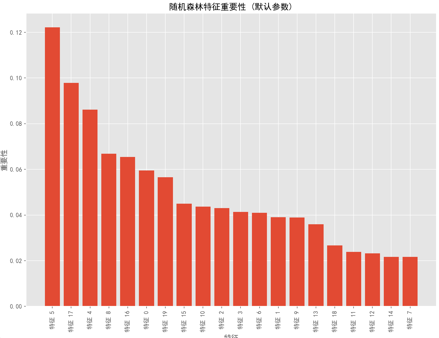
)try:grid_search_coarse.fit(X_train, y_train)coarse_time = time.time() - start_timeprint(f"\n粗调参数完成，耗时: {coarse_time:.2f}秒")print(f"最佳参数组合: {grid_search_coarse.best_params_}")print(f"最佳交叉验证准确率: {grid_search_coarse.best_score_:.4f}")# 6. 基于粗调结果进行精调print("\n[步骤6] 基于粗调结果定义精调参数网格...")# 从粗调中获取最佳参数best_n_estimators = grid_search_coarse.best_params_['n_estimators']best_max_depth = grid_search_coarse.best_params_['max_depth']best_min_samples_split = grid_search_coarse.best_params_['min_samples_split']best_min_samples_leaf = grid_search_coarse.best_params_['min_samples_leaf']best_max_features = grid_search_coarse.best_params_['max_features']# 根据粗调结果定义更精细的参数网格 - 简化版本param_grid_fine = {'n_estimators': [best_n_estimators, best_n_estimators + 50],'max_features': [best_max_features],}# 对max_depth特别处理if best_max_depth is None:param_grid_fine['max_depth'] = [None, 15]else:param_grid_fine['max_depth'] = [best_max_depth, best_max_depth + 5]# 添加其他参数的精细搜索param_grid_fine['min_samples_split'] = [best_min_samples_split, best_min_samples_split + 1]param_grid_fine['min_samples_leaf'] = [best_min_samples_leaf, best_min_samples_leaf + 1]# 添加其他可能影响性能的参数param_grid_fine['bootstrap'] = [True]param_grid_fine['criterion'] = ['gini', 'entropy']print("精调参数网格:")for param, values in param_grid_fine.items():print(f"- {param}: {values}")# 7. 执行精调网格搜索print("\n[步骤7] 执行精调参数的网格搜索(可能需要较长时间)...")start_time = time.time()grid_search_fine = GridSearchCV(estimator=rf_base,param_grid=param_grid_fine,scoring='accuracy',cv=3,                  # 3折交叉验证，加快速度n_jobs=-1,verbose=1,return_train_score=True)grid_search_fine.fit(X_train, y_train)fine_time = time.time() - start_timeprint(f"\n精调参数完成，耗时: {fine_time:.2f}秒")print(f"最终最佳参数组合: {grid_search_fine.best_params_}")print(f"最终最佳交叉验证准确率: {grid_search_fine.best_score_:.4f}")# 8. 使用最佳参数评估模型print("\n[步骤8] 使用最佳参数评估模型性能...")best_rf = grid_search_fine.best_estimator_y_pred = best_rf.predict(X_test)accuracy = accuracy_score(y_test, y_pred)print(f"测试集准确率: {accuracy:.4f}")print("\n分类报告:")print(classification_report(y_test, y_pred))# 9. 可视化结果print("\n[步骤9] 可视化评估结果...")# 9.1 混淆矩阵plt.figure(figsize=(10, 8))cm = confusion_matrix(y_test, y_pred)sns.heatmap(cm, annot=True, fmt='d', cmap='Blues')plt.title('随机森林最佳模型混淆矩阵', fontsize=14)plt.xlabel('预测标签', fontsize=12)plt.ylabel('真实标签', fontsize=12)if chinese_font:plt.title('随机森林最佳模型混淆矩阵', fontproperties=chinese_font, fontsize=14)plt.xlabel('预测标签', fontproperties=chinese_font, fontsize=12)plt.ylabel('真实标签', fontproperties=chinese_font, fontsize=12)plt.tight_layout()plt.savefig('rf_confusion_matrix.png', dpi=300, bbox_inches='tight')plt.show()# 9.2 ROC曲线plt.figure(figsize=(10, 8))y_scores = best_rf.predict_proba(X_test)[:, 1]fpr, tpr, _ = roc_curve(y_test, y_scores)roc_auc = auc(fpr, tpr)plt.plot(fpr, tpr, color='darkorange', lw=2, label=f'ROC曲线 (AUC = {roc_auc:.3f})')plt.plot([0, 1], [0, 1], color='navy', lw=2, linestyle='--')plt.xlim([0.0, 1.0])plt.ylim([0.0, 1.05])plt.xlabel('假阳性率', fontsize=12)plt.ylabel('真阳性率', fontsize=12)plt.title('随机森林最佳模型ROC曲线', fontsize=14)plt.legend(loc="lower right")if chinese_font:plt.xlabel('假阳性率', fontproperties=chinese_font, fontsize=12)plt.ylabel('真阳性率', fontproperties=chinese_font, fontsize=12)plt.title('随机森林最佳模型ROC曲线', fontproperties=chinese_font, fontsize=14)for text in plt.legend().get_texts():text.set_fontproperties(chinese_font)plt.tight_layout()plt.savefig('rf_roc_curve.png', dpi=300, bbox_inches='tight')plt.show()# 9.3 特征重要性plt.figure(figsize=(12, 10))importances = best_rf.feature_importances_indices = np.argsort(importances)[::-1]plt.bar(range(X_train.shape[1]), importances[indices], align='center')plt.xticks(range(X_train.shape[1]), [f'特征 {i}' for i in indices], rotation=90)plt.title('随机森林特征重要性', fontsize=14)plt.xlabel('特征', fontsize=12)plt.ylabel('重要性', fontsize=12)if chinese_font:plt.title('随机森林特征重要性', fontproperties=chinese_font, fontsize=14)plt.xlabel('特征', fontproperties=chinese_font, fontsize=12)plt.ylabel('重要性', fontproperties=chinese_font, fontsize=12)plt.xticks(rotation=90, fontproperties=chinese_font)plt.tight_layout()plt.savefig('rf_feature_importance.png', dpi=300, bbox_inches='tight')plt.show()# 9.4 参数重要性def plot_param_importance(grid_search, title):plt.figure(figsize=(14, 10))results = pd.DataFrame(grid_search.cv_results_)# 提取参数名称param_names = [p for p in results.columns if p.startswith('param_')]# 创建一个包含每个参数的单独子图n_params = len(param_names)n_cols = 2n_rows = (n_params + 1) // 2for i, param_name in enumerate(param_names):plt.subplot(n_rows, n_cols, i + 1)# 提取参数的实际名称(不含"param_"前缀)param = param_name[6:]# 获取参数值和对应的平均测试分数param_values = results[param_name].astype(str)unique_values = param_values.unique()# 对于每个唯一的参数值，计算其平均测试分数mean_scores = [results[param_values == val]['mean_test_score'].mean() for val in unique_values]# 创建条形图plt.bar(range(len(unique_values)), mean_scores)plt.xticks(range(len(unique_values)), unique_values, rotation=45)plt.title(f'参数 {param} 的影响', fontsize=12)plt.xlabel(param, fontsize=10)plt.ylabel('平均测试分数', fontsize=10)if chinese_font:plt.title(f'参数 {param} 的影响', fontproperties=chinese_font, fontsize=12)plt.xlabel(param, fontproperties=chinese_font, fontsize=10)plt.ylabel('平均测试分数', fontproperties=chinese_font, fontsize=10)plt.suptitle(title, fontsize=16)if chinese_font:plt.suptitle(title, fontproperties=chinese_font, fontsize=16)plt.tight_layout(rect=[0, 0, 1, 0.96])plt.savefig('rf_param_importance.png', dpi=300, bbox_inches='tight')plt.show()# 显示精调参数的重要性plot_param_importance(grid_search_fine, '随机森林参数重要性分析')# 9.5 学习曲线train_sizes, train_scores, test_scores = learning_curve(best_rf, X_train, y_train, cv=3, n_jobs=-1,train_sizes=np.linspace(0.1, 1.0, 5)  # 减少点数以加快速度)train_mean = np.mean(train_scores, axis=1)train_std = np.std(train_scores, axis=1)test_mean = np.mean(test_scores, axis=1)test_std = np.std(test_scores, axis=1)plt.figure(figsize=(10, 8))plt.plot(train_sizes, train_mean, color='blue', marker='o', markersize=5, label='训练集分数')plt.fill_between(train_sizes, train_mean + train_std, train_mean - train_std, alpha=0.15, color='blue')plt.plot(train_sizes, test_mean, color='green', marker='s', markersize=5, label='验证集分数')plt.fill_between(train_sizes, test_mean + test_std, test_mean - test_std, alpha=0.15, color='green')plt.title('随机森林最佳模型学习曲线', fontsize=14)plt.xlabel('训练样本数', fontsize=12)plt.ylabel('准确率', fontsize=12)plt.grid(True)plt.legend(loc='lower right')if chinese_font:plt.title('随机森林最佳模型学习曲线', fontproperties=chinese_font, fontsize=14)plt.xlabel('训练样本数', fontproperties=chinese_font, fontsize=12)plt.ylabel('准确率', fontproperties=chinese_font, fontsize=12)for text in plt.legend().get_texts():text.set_fontproperties(chinese_font)plt.tight_layout()plt.savefig('rf_learning_curve.png', dpi=300, bbox_inches='tight')plt.show()# 10. 总结最佳模型配置print("\n[步骤10] 最终随机森林模型配置:")for param, value in best_rf.get_params().items():print(f"- {param}: {value}")print("\n超参数调优实验完成！")print(f"总耗时: {coarse_time + fine_time:.2f}秒")print(f"最终模型测试集准确率: {accuracy:.4f}")except Exception as e:print(f"发生错误: {str(e)}")print("尝试不使用并行处理的简化版本...")# 如果并行处理失败，尝试使用简化版本（不使用并行）rf_base = RandomForestClassifier(n_estimators=100,max_depth=10,min_samples_split=2,min_samples_leaf=1,max_features='sqrt',random_state=42)rf_base.fit(X_train, y_train)y_pred = rf_base.predict(X_test)accuracy = accuracy_score(y_test, y_pred)print(f"\n使用默认参数的随机森林模型准确率: {accuracy:.4f}")print("\n分类报告:")print(classification_report(y_test, y_pred))# 简单的可视化plt.figure(figsize=(12, 10))importances = rf_base.feature_importances_indices = np.argsort(importances)[::-1]plt.bar(range(X_train.shape[1]), importances[indices], align='center')plt.xticks(range(X_train.shape[1]), [f'特征 {i}' for i in indices], rotation=90)plt.title('随机森林特征重要性 (默认参数)', fontsize=14)plt.xlabel('特征', fontsize=12)plt.ylabel('重要性', fontsize=12)if chinese_font:plt.title('随机森林特征重要性 (默认参数)', fontproperties=chinese_font, fontsize=14)plt.xlabel('特征', fontproperties=chinese_font, fontsize=12)plt.ylabel('重要性', fontproperties=chinese_font, fontsize=12)plt.xticks(rotation=90, fontproperties=chinese_font)plt.tight_layout()plt.savefig('rf_feature_importance_default.png', dpi=300, bbox_inches='tight')plt.show()finally:# 清理临时文件夹import shutiltry:shutil.rmtree(temp_dir)print(f"已清理临时文件夹: {temp_dir}")except:pass

程序运行结果如下：

临时文件夹路径: C:\Users\ABC\AppData\Local\Temp\sklearn_rf_iyndeds8
使用字体: C:/Windows/Fonts/simhei.ttf
随机森林超参数调优实验
--------------------------------------------------

[步骤1] 生成分类数据集...
[步骤2] 划分训练集和测试集...
训练集大小: (800, 20)
测试集大小: (200, 20)
特征数量: 20

[步骤3] 定义参数网格...
粗调参数网格:
- n_estimators: [50, 100]
- max_depth: [None, 10]
- min_samples_split: [2, 5]
- min_samples_leaf: [1, 2]
- max_features: ['sqrt', 'log2']

[步骤4] 创建基础随机森林模型...

[步骤5] 执行粗调参数的网格搜索(可能需要较长时间)...
发生错误: 'ascii' codec can't encode characters in position 18-20: ordinal not in range(128)
尝试不使用并行处理的简化版本...

使用默认参数的随机森林模型准确率: 0.8850

分类报告:
precision recall f1-score support

0 0.91 0.84 0.87 93
1 0.87 0.93 0.90 107

accuracy 0.89 200
macro avg 0.89 0.88 0.88 200
weighted avg 0.89 0.89 0.88 200