@浙大疏锦行

对于数据的认识，很重要的一点是，很多数据并非是为了某个确定的问题收集的，这也意味着一份数据你可以完成很多不同的研究， 自变量、因变量的选取取决于你自己-----很多时候针对现有数据的思考才是真正拉开你与他人差距的最重要因素。

现在可以发现，其实掌握流程后，机器学习项目流程是比较固定的，对于掌握的同学来说，工作量非常少。所以这也是很多论文被懂的认为比较水的原因所在。所以这类研究真正核心的地方集中在以下几点：

1. 数据的质量上，是否有好的研究主题但是你这个数据很难获取，所以你这个研究有价值
2. 研究问题的选择上，同一个数据你找到了有意思的点，比如更换了因变量，做出了和别人不同的研究问题
3. 同一个问题，特征加工上，是否对数据进一步加工得出了新的结论-----你的加工被证明是有意义的。

后续我们会不断给出，在现有框架上，如何加大工作量的思路。

一些数据集平台：

GitHub开源数据集 国外平台，最好科学上网

kaggle开源数据集 国外平台，下载浏览器插件注册，数据集质量自己筛选

天池开源数据集 阿里平台，电商类数据集较多

和鲸开源数据集 国内平台，包含经典的数据集

用到的数据集：机器故障数据集

说明：1.该数据集全是数值型，没有字符串等分类型信息

        2.该数据集中没有缺失值

        3.数据集信息

名称	说明
footfall	经过机器的人数或物体数量
tempMode	机器的温度模式或设置
AQ	机器附近的空气质量指数
USS	超声波传感器数据，表示接近度测量
CS	当前传感器读数，表示机器的电流使用情况
VOC	检测到的挥发性有机化合物水平
RP	机器部件的旋转位置或每分钟转数
IP	机器的输入压力
Temperature	机器的运行温度
fail	机器故障的二元指示器（1表示故障，0表示无故障）

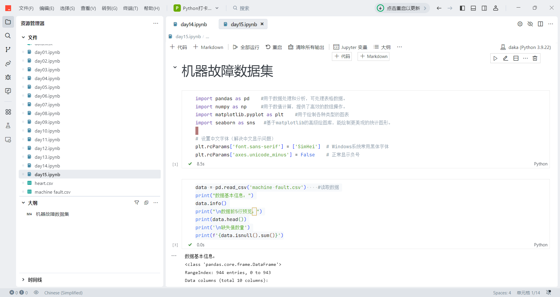
import pandas as pd    #用于数据处理和分析，可处理表格数据。
import numpy as np     #用于数值计算，提供了高效的数组操作。
import matplotlib.pyplot as plt    #用于绘制各种类型的图表
import seaborn as sns   #基于matplotlib的高级绘图库，能绘制更美观的统计图形。# 设置中文字体（解决中文显示问题）
plt.rcParams['font.sans-serif'] = ['SimHei']  # Windows系统常用黑体字体
plt.rcParams['axes.unicode_minus'] = False    # 正常显示负号

data = pd.read_csv('machine fault.csv')    #读取数据
print("数据基本信息：")
data.info()
print("\n数据前5行预览：")
print(data.head())
print('\n缺失值数量')
print(f'{data.isnull().sum()}')

数据基本信息：
<class 'pandas.core.frame.DataFrame'>
RangeIndex: 944 entries, 0 to 943
Data columns (total 10 columns):
 #   Column       Non-Null Count  Dtype
---  ------       --------------  -----
 0   footfall     944 non-null    int64
 1   tempMode     944 non-null    int64
 2   AQ           944 non-null    int64
 3   USS          944 non-null    int64
 4   CS           944 non-null    int64
 5   VOC          944 non-null    int64
 6   RP           944 non-null    int64
 7   IP           944 non-null    int64
 8   Temperature  944 non-null    int64
 9   fail         944 non-null    int64
dtypes: int64(10)
memory usage: 73.9 KB

数据前5行预览：
   footfall  tempMode  AQ  USS  CS  VOC  RP  IP  Temperature  fail
0         0         7   7    1   6    6  36   3            1     1
1       190         1   3    3   5    1  20   4            1     0
2        31         7   2    2   6    1  24   6            1     0
3        83         4   3    4   5    1  28   6            1     0
4       640         7   5    6   4    0  68   6            1     0

缺失值数量
footfall       0
tempMode       0
AQ             0
USS            0
CS             0
VOC            0
RP             0
IP             0
Temperature    0
fail           0
dtype: int64

continuous_features = data.select_dtypes(include=['float64','int64']).columns.tolist()
for col in continuous_features:plt.figure(figsize=(8, 6))sns.histplot(x=data[col])plt.title(f'{col} 直方图')plt.xlabel(col)plt.show()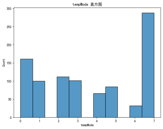

 

# 借助sklearn库进行归一化
from sklearn.preprocessing import StandardScaler, MinMaxScaler# 拆分离散特征和连续特征
discrete_features = data.select_dtypes(include=['object']).columns.tolist()
continuous_features = data.select_dtypes(include=['float64','int64']).columns.tolist()# 归一化处理
min_max_scaler = MinMaxScaler() # 实例化 MinMaxScaler
min_max_columns=['RP','Temperature']
for col in min_max_columns:data[col] = min_max_scaler.fit_transform(data[[col]])# 标准化
scaler = StandardScaler() # 实例化 StandardScaler类
standard_columns=['footfall']
for col in standard_columns:data[col] = min_max_scaler.fit_transform(data[[col]])

# 热力图
# corr()函数，用于计算相关系数矩阵
correlation_matrix = data[continuous_features].corr()# 设置图片清晰度
plt.rcParams['figure.dpi'] = 500# 绘制热力图
plt.figure(figsize=(10, 8))   # 画布中小格子的大小
sns.heatmap(correlation_matrix, annot=True, cmap='coolwarm', vmin=-1, vmax=1)
plt.title('连续特征的相关系数热力图')
plt.xticks(rotation=45)#横坐标旋转45度# 调整子图布局，增加左右边距
plt.subplots_adjust(left=0.2, right=0.8)
plt.show()#子图
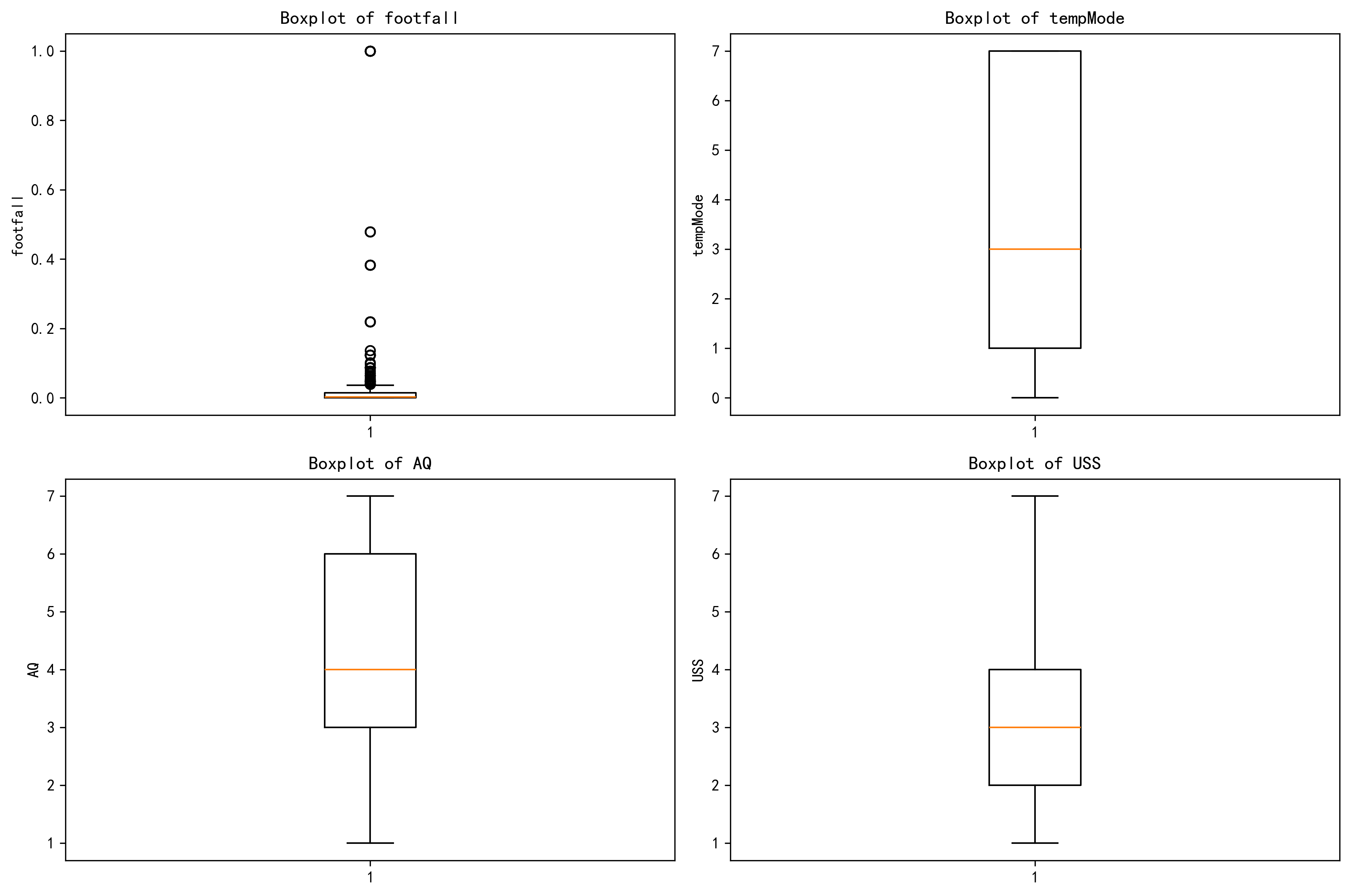
# 定义要绘制的特征
features = ['footfall', 'tempMode', 'AQ', 'USS']# 设置图片清晰度
plt.rcParams['figure.dpi'] = 300# 创建一个包含 2 行 2 列的子图布局，并设置每个图形大小
fig, axes = plt.subplots(2, 2, figsize=(12, 8))# 使用 for 循环遍历特征
for i in range(len(features)):row = i // 2 # // 是整除，即取整 ，取整获得特征在子图中的行位置col = i % 2 # % 是取余，取余获得特征在子图中的列位置# 绘制箱线图feature = features[i]axes[row, col].boxplot(data[feature].dropna())axes[row, col].set_title(f'Boxplot of {feature}')axes[row, col].set_ylabel(feature)# 调整子图之间的间距
plt.tight_layout()# 显示图形
plt.show()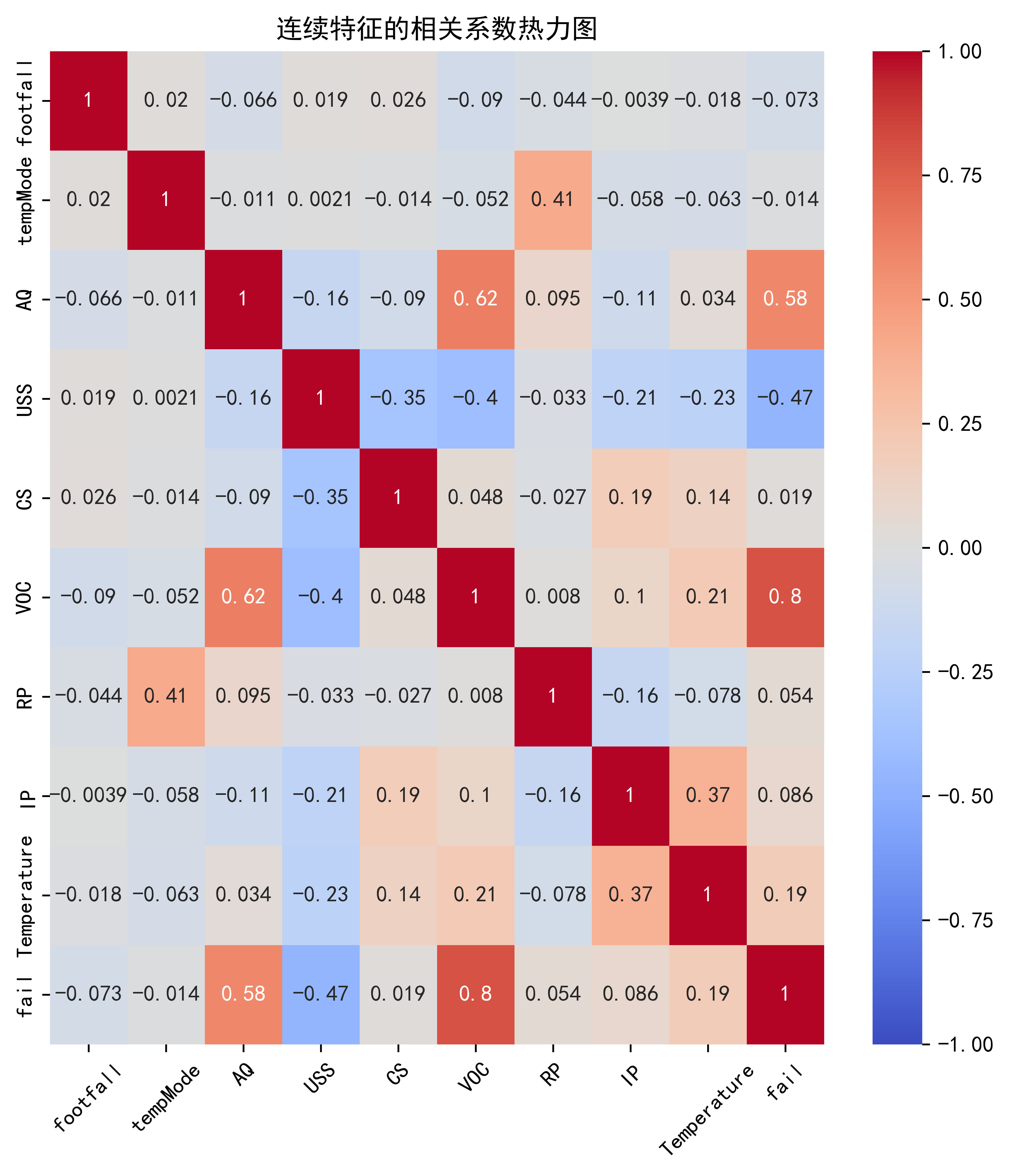

 

# 划分训练集和测试机
from sklearn.model_selection import train_test_split
X = data.drop(['fail'], axis=1)  # 定义特征列，axis=1表示按列删除
y = data['fail']  # 标签
X_train, X_test, y_train, y_test = train_test_split(X, y, test_size=0.2, random_state=42)  # 划分数据集，20%作为测试集，随机种子为42
# 训练集和测试集的形状
print(f"训练集特征形状: {X_train.shape}, 测试集特征形状: {X_test.shape}")  # 打印训练集和测试集的形状
print(f'标签形状{y_train.shape}')

训练集特征形状: (755, 9), 测试集特征形状: (189, 9)
标签形状(755,)

from sklearn.svm import SVC #支持向量机分类器
from sklearn.neighbors import KNeighborsClassifier #K近邻分类器
from sklearn.linear_model import LogisticRegression #逻辑回归分类器
import xgboost as xgb #XGBoost分类器
import lightgbm as lgb #LightGBM分类器
from sklearn.ensemble import RandomForestClassifier #随机森林分类器
from catboost import CatBoostClassifier #CatBoost分类器
from sklearn.tree import DecisionTreeClassifier #决策树分类器
from sklearn.naive_bayes import GaussianNB #高斯朴素贝叶斯分类器from sklearn.metrics import accuracy_score, precision_score, recall_score, f1_score # 用于评估分类器性能的指标
from sklearn.metrics import classification_report, confusion_matrix #用于生成分类报告和混淆矩阵
import warnings #用于忽略警告信息
warnings.filterwarnings("ignore") # 忽略所有警告信息

print("--- 1. 默认参数随机森林 (训练集 -> 测试集) ---")
import time # 这里介绍一个新的库，time库，主要用于时间相关的操作，因为调参需要很长时间，记录下会帮助后人知道大概的时长start_time = time.time() # 记录开始时间
rf_model = RandomForestClassifier(random_state=42)#模型实例化
rf_model.fit(X_train, y_train) # 在训练集上训练
rf_pred = rf_model.predict(X_test) # 在测试集上预测
end_time = time.time() # 记录结束时间print(f"训练与预测耗时: {end_time - start_time:.4f} 秒")
print("\n默认随机森林 在测试集上的分类报告：")
print(classification_report(y_test, rf_pred))
print("默认随机森林 在测试集上的混淆矩阵：")
print(confusion_matrix(y_test, rf_pred))

--- 1. 默认参数随机森林 (训练集 -> 测试集) ---
训练与预测耗时: 0.1943 秒

默认随机森林 在测试集上的分类报告：
              precision    recall  f1-score   support

           0       0.89      0.88      0.89       102
           1       0.86      0.87      0.87        87

    accuracy                           0.88       189
   macro avg       0.88      0.88      0.88       189
weighted avg       0.88      0.88      0.88       189

默认随机森林 在测试集上的混淆矩阵：
[[90 12]
 [11 76]]

# SMOTE过采样
from imblearn.over_sampling import SMOTE 
smote = SMOTE(random_state=42)
X_train_smote, y_train_smote = smote.fit_resample(X_train, y_train)print("SMOTE过采样后训练集的形状：", X_train_smote.shape, y_train_smote.shape)# 训练随机森林模型（使用SMOTE过采样后的训练集）
rf_model_smote = RandomForestClassifier(random_state=42)
start_time_smote = time.time()
rf_model_smote.fit(X_train_smote, y_train_smote)
end_time_smote = time.time()print(f"SMOTE过采样后训练与预测耗时: {end_time_smote - start_time_smote:.4f} 秒")# 在测试集上预测
rf_pred_smote = rf_model_smote.predict(X_test)print("\nSMOTE过采样后随机森林 在测试集上的分类报告：")
print(classification_report(y_test, rf_pred_smote))
print("SMOTE过采样后随机森林 在测试集上的混淆矩阵：")
print(confusion_matrix(y_test, rf_pred_smote))

SMOTE过采样后训练集的形状： (898, 9) (898,)
SMOTE过采样后训练与预测耗时: 0.1721 秒

SMOTE过采样后随机森林 在测试集上的分类报告：
              precision    recall  f1-score   support

           0       0.89      0.87      0.88       102
           1       0.85      0.87      0.86        87

    accuracy                           0.87       189
   macro avg       0.87      0.87      0.87       189
weighted avg       0.87      0.87      0.87       189

SMOTE过采样后随机森林 在测试集上的混淆矩阵：
[[89 13]
 [11 76]]

print("\n--- 2. 网格搜索优化随机森林 (训练集 -> 测试集) ---")
from sklearn.model_selection import GridSearchCV# 定义要搜索的参数网格
param_grid = {'n_estimators': [50, 100, 200],'max_depth': [None, 10, 20, 30],'min_samples_split': [2, 5, 10],'min_samples_leaf': [1, 2, 4]
}# 创建网格搜索对象
grid_search = GridSearchCV(estimator=RandomForestClassifier(random_state=42), # 随机森林分类器param_grid=param_grid, # 参数网格cv=5, # 5折交叉验证n_jobs=2, # 使用所有可用的CPU核心进行并行计算scoring='accuracy') # 使用准确率作为评分标准start_time = time.time()
# 在训练集上进行网格搜索
grid_search.fit(X_train, y_train) # 在训练集上训练，模型实例化和训练的方法都被封装在这个网格搜索对象里了
end_time = time.time()print(f"网格搜索耗时: {end_time - start_time:.4f} 秒")
print("最佳参数: ", grid_search.best_params_) #best_params_属性返回最佳参数组合# 使用最佳参数的模型进行预测
best_model = grid_search.best_estimator_ # 获取最佳模型
best_pred = best_model.predict(X_test) # 在测试集上进行预测print("\n网格搜索优化后的随机森林 在测试集上的分类报告：")
print(classification_report(y_test, best_pred))
print("网格搜索优化后的随机森林 在测试集上的混淆矩阵：")
print(confusion_matrix(y_test, best_pred))

--- 2. 网格搜索优化随机森林 (训练集 -> 测试集) ---
网格搜索耗时: 50.6869 秒
最佳参数:  {'max_depth': 10, 'min_samples_leaf': 2, 'min_samples_split': 5, 'n_estimators': 100}

网格搜索优化后的随机森林 在测试集上的分类报告：
              precision    recall  f1-score   support

           0       0.91      0.87      0.89       102
           1       0.86      0.90      0.88        87

    accuracy                           0.88       189
   macro avg       0.88      0.88      0.88       189
weighted avg       0.88      0.88      0.88       189

网格搜索优化后的随机森林 在测试集上的混淆矩阵：
[[89 13]
 [ 9 78]]

import shap
# 初始化 SHAP 解释器
explainer = shap.TreeExplainer(rf_model)
shap_values = explainer.shap_values(X_test)print('展示特征维度')
print("shap_values 的形状:", shap_values.shape)
print("shap_values[0] 的形状:", shap_values[0].shape)
print("shap_values[:, :, 0] 的形状:", shap_values[:, :, 0].shape)
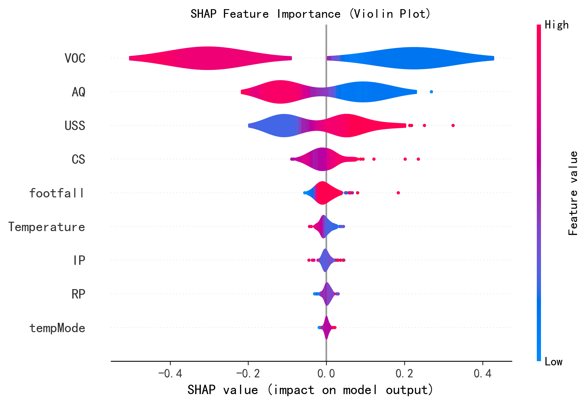
print("X_test 的形状:", X_test.shape)print("--- SHAP 特征重要性蜂巢图 ---")
shap.summary_plot(shap_values[:, :, 0], X_test,plot_type="violin",show=False,max_display=10) # 这里的show=False表示不直接显示图形,这样可以继续用plt来修改元素，不然就直接输出了
plt.title("SHAP Feature Importance (Violin Plot)")
plt.show()
print("---  SHAP 决策图 ---")
shap.decision_plot(explainer.expected_value[0], shap_values[0,:,0], X_test.iloc[0], #feature_order='hclust',show=False)
plt.title("SHAP Decision Plot")
plt.show()

展示特征维度
shap_values 的形状: (189, 9, 2)
shap_values[0] 的形状: (9, 2)
shap_values[:, :, 0] 的形状: (189, 9)
X_test 的形状: (189, 9)
--- SHAP 特征重要性蜂巢图 --- 

代码实现